In my previous article on streaming in Spark, we looked at some of the less obvious fine points of grouping via time windows, the interplay between triggers and processing time, and processing time vs. event time. This article will look at some related topics and contrast the older DStream-based API with the newer (and officially recommended) Structured Streaming API via an exploration of how we might rewrite an existing DStream based application using the newer API, with particular focus on sliding windows.
The first section of the article builds some intuition around slide intervals, windows, and the events they can potentially ‘subsume’ (definition to follow). Then we discuss some key differences between DStream and Structured Streaming-based processing, present a motivating use case, and then dive into some code. The final section provides a rigorous proof of some of the claims made in the first section.
Sliding Windows Intuition
Do any patterns emerge when we look at how the timestamped events ingested into our applications are bucketed to particular windows in a series of sliding windows across some time line? Are there any structural patterns that we can use to classify the types of windows into which our events fall? There are indeed, and we will explore those patterns here. (Sliding windows are discussed at a general level in both the DStream programming documentation — in the subsection entitled Window Operations of this section, and in the Structured Streaming guide.)
When we write unit tests or spot check the results of our application code, there will always be some bounded time interval (let’s call it I) that ‘brackets’ the timestamps of the earliest and latest incoming events in our test set. Clearly, we care what’s happening with events inside of I, not outside of it. It would also be helpful to know, given our test set and how we choose I, these two things: (a) the number of windows we must consider when checking our results (here a must consider window is one which could potentially subsume an incoming event) , and (b) for any specific event, e, in our test set, how many windows will subsume e. When a window, w, subsumes an event e, the following must hold: startTime(w) <= timestamp(e) < endTime(w).
Reasoning will be easier if we make the simplifying assumptions that
- our window length w is equal to some integral multiple k (k >= 1) of our slide interval, s,
- our interval I begins at zero, and is equal to some integral multiple n (n >= 1) of w. (This means s < w < I, s*k =w, and n*w=I)
We shall see shortly that we must consider some windows which are not completely contained within I: in particular, we will see that some of our events are subsumed within what we call overlapping windows – those whose start time stamp is less than the time stamp that marks the start of I (but whose end time stamp lies within I), and those whose end time stamp is greater than the time stamp that marks the end of I (but whose start time stamp lies within I.) We will also provide a proof that the total number of windows we must consider is k + kn – 1, the total number of completely contained windows is kn – k + 1, and the total number of overlapping windows is 2(k-1).
For now, we will show how these formulas work via an example where our time units are in seconds (although the formula can also be applied when developing applications that work in terms of finer or coarser grained units (e.g., milliseconds as we get more fine grained, or hours or days as the granularity of our bucketing gets coarser.) In our example the window interval (W) is set to 30 seconds, the slide interval (S) is set to 15 seconds, and the time interval I which bounds the earliest and latest arriving events is set to 60 seconds. Given these values, n = 2, and k = 2.
I = 60
W = 30
S = 15
   where n and k = 2, since  W (30) = 2 * S (15), and I (60) = 2 * W
In the diagram below there are a total of 5 must consider windows (w1 through w5, in green), and this is the same number that our formula gives us:
cardinality (must consider windows) = k + kn - 1
= 2 + 2*2 - 1
= 2 + 4 - 1 = 5
The total number of overlapping and completely contained windows is 2 (w1 and w5), and 3 (w2 – w5) respectively. These results accord with the cardinality formulas for these two window types:
cardinality (overlapping windows) = 2 * (k -1)
= 2 * (2 - 1)
= 2 * 1 = 2

cardinality (completely contained windows) = k * n - k + 1
= 2 * 2 - 2 + 1
= 4 - 1 =  3
k Windows Will Always Subsume An Arbitrary Point
Here we make the claim that for any arbitrary point, p, on the half-open Interval I’ from 0 (inclusive) to I (exclusive) there are k windows that subsume p. In this article we will not offer a formal mathematical proof, but will instead illustrate with two examples. First off, referring to the diagram above, pick a point on I’ (e.g., x, or y, or any other point you prefer,) then note that the chosen point will fall within 2 windows (and also note that, for the scenario illustrated in the above diagram, k = 2.) For a more general example, refer to the diagram below. This diagram shows windows of length w, where w is k times the slide interval. We have selected an arbitrary point p within I’ and we see that it is subsumed by (among other windows) window w_1, where it lies in the i-th slide segment (a term which we haven’t defined, but whose meaning should be intuitively obvious.)
Visually, it seems clear that we can forward slide w_1 i – 1 times and still have p subsumed by window w_1. After the i-th slide the startTime of the resultant window would be greater than p. Similarly we could backward slide w_1 k – i times and still have p subsumed by the result of the slide. After the (k – i + 1)th backward slide the endTime of the resultant window would be less than p. This makes for a total of 1 + (i – 1) + (k – i) position variations of w_1 that will subsume point p (we add one to account for the original position of w_1.) Arranging like terms, we have 1 – 1 + i – i + k = k possible variants. Each of these variants would map to one of w actual windows that would subsume point p. So this illustrates the general case.
Key Differences In How The Two Frameworks Handle Windows
Now let’s move from more abstract concepts towards a discussion of some key high level differences between the two frameworks we will be examining. First we note that DStream sliding windows are based on processing time – the time of an event’s arrival into the framework, whereas Structured Streaming sliding windows are based on the timestamp value of one of the attributes of incoming event records. Such timestamp attributes are usually set by the source system that generated the original event; however, you can also base your Structured Streaming logic on processing time by targeting an attribute whose value is generated by the current_time stamp function.
So with DStreams the timestamps of the windows that will subsume your test events will be determined by your system clock, whereas with Structured Streaming these factors are ‘preordained’ by one of the timestamp-typed attributes of those events. Fortunately, for DStreams there are some libraries — such as Holden Karau’s Spark Testing Base that let you write unit tests using a mock system clock, with the result that you obtain more easily reproducible results. This is less of a help when you are spot checking the output of your non-test code, however. In these cases each run will bucket your data into windows with different timestamps.
By contrast, Structured Streaming will always bucket the same test data into the same windows (again, provided the timestamps on your test events are not generated via current_timestamp — but even if they are you can always mock that data using fixed timestamps.) This makes it much easier to write tests and spot check results of non-test code, since you can more reliably reproduce the same results. You can also prototype the code you use to process your event data using non-streaming batch code (using the typed Dataset API, or Dataframes with sparkSession.read.xxx, instead of sparkSession.readStream.xxx). But note that not every series of transformations that you can apply in batch is guaranteed to work when you move to streaming. An example of something that won’t transfer well (unless you use a trick that we reveal later) is code that uses chained aggregations, as discussed here.
A final key difference we will note is that, with DStreams, once a sliding window’s end time is reached no subsequently arriving events can be bucketed to that window (without significant extra work.) The original DStreams paper does attempt to address this by sketching (in section 3.2, Timing Considerations) two approaches to handling late arriving data, neither of which seems totally satisfactory. The first is to simply wait for some “slack time” before processing each batch (which would increase end-to-end latency), and the second is to correct late records at the application level, which seems to suggest foregoing the convenience of built in (arrival time-based) window processing features, and instead managing window state by hand.
Structured Streams supports updating previously output windows with late arriving data by design. You can set limits on how long you will wait for late arriving data using watermarks, which we don’t have space to explore in much detail here. However, you can refer to the section Watermarking to Limit State while Handling Late Data of this blog post for a pictorial walk through of how the totals of a previously output window are updated with late arriving data (pay particular attention to the totals for ‘dev2’ in window 12:00-12:10). The ability to handle late arriving data can be quite useful in cases where sources that feed into your application might be intermittently connected, such as if you were getting sensor data from vehicles which might, at some point, pass through a tunnel (in which case older data would build up and be transmitted in a burst. )
Motivating Use Case
We’ll look at code shortly, but let us first discuss our use case. We are going to suppose we work for a company that has deployed a variety of sensors across some geographic area and our boss wants us to create a dashboard that shows, for each type of sensor, what the top state of that sensor type is across all sensors in all regions, and across some sliding time window (assuming that, at any point in time, a given sensor can be in exactly one out of some finite set of states.) Whether we are working with DStreams or Structured Streams the basic approach will be to monitor a directory for incoming text files, each of which contain event records of the form:
<ISO 8601 timestamp>,<sensorType>,<region>,<commaSeparatedStateList>
At any given time the program that sends us events will poll all sensors in the region, and some subset will respond with their states. For the sake of this toy example, we assume that if the sender found multiple sensors with the same state (say 3) within some polling interval, then the message it transmits will have X repeated 3 times, resulting in an event that would look something like the line below.
2008-09-15T15:53:00,temp,london,X,X,XOur toy program will also simply zero in on sensors of type ‘temp’ and will punt on aggregating along the dimension of sensor type.
How We Test The Two Solutions
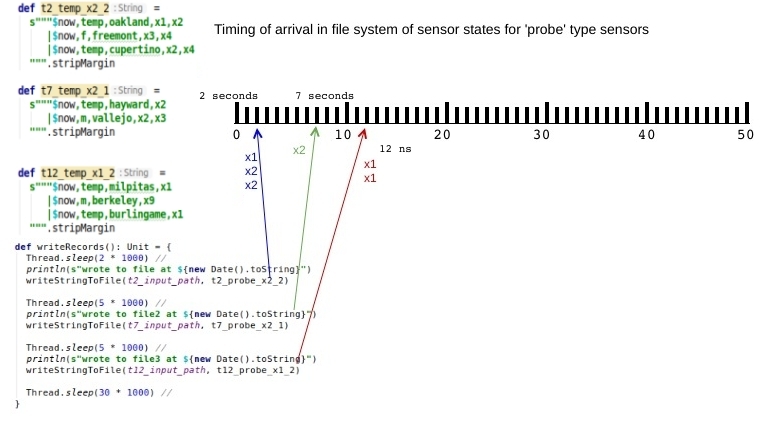
The solutions we developed with both the old and new API need to pass the same test scenario. This scenario involves writing out files containing sensor events to a monitored directory, in batches that are sequenced in time as per the diagram below.
Both solution approaches will bucket incoming events into 30 second windows, with a slide interval of 10 seconds, and then write out the the top most frequently occurring events using the formatting below (out of laziness we opted to output the toString representation of the data structure we use to track the top events):
for window 2019-06-29 11:27:00.0 got sensor states: TreeSet(x2)
for window 2019-06-29 11:27:10.0 got sensor states: TreeSet(x1, x2)
The next diagram we present shows the code that writes out event batches at 2, 7, and 12 seconds. Note that each call to writeStringToFile is associated with a color coded set of events that matches the color coding in the first diagram presented in this section.
The main flow of the test that exercises both solutions is shown below, while the full listing of our test code is available here.
  "Top Sensor State Reporter" should {
    "correctly output top states for target sensor using DStreams" in {
      setup()

      val ctx: StreamingContext =
        new DstreamTopSensorState().
          beginProcessingInputStream(
            checkpointDirPath, incomingFilesDirPath, outputFile)

      writeRecords()
      verifyResult
      ctx.stop()
    }

    "correctly output top states for target sensor using structured streaming" in {
      import com.lackey.stream.examples.dataset.StreamWriterStrategies._

      setup()

      val query =
        StructuredStreamingTopSensorState.
          processInputStream(doWrites = fileWriter)

      writeRecords()
      verifyResult
      query.stop()
    }
  }
DStreams Approach WALK-THROUGH
The main entry point to the DStream solution is beginProcessingInputStream(), which takes a checkpoint directory, the path of the directory to monitor for input, and the path of the file where we write final results.
def beginProcessingInputStream(checkpointDirPath: String,

                                 incomingFilesDirPath: String,

                                 outputFile: String): StreamingContext = {

    val ssc = StreamingContext.

      getOrCreate(

        checkpointDirPath,

        () => createContext(incomingFilesDirPath, checkpointDirPath, outputFile))

    ssc.start()

    ssc

  }
Note the above method invokes StreamingContext.getOrCreate(), passing, as the second argument, a function block which invokes the method which will actually create the context, shown below
def createContext(incomingFilesDir: String,
                     checkpointDirectory: String,
                     outputFile: String): StreamingContext = {
     val sparkConf = new SparkConf().setMaster("local[*]").setAppName("OldSchoolStreaming")
     val ssc = new StreamingContext(sparkConf, BATCH_DURATION)
     ssc.checkpoint(checkpointDirectory)
     ssc.sparkContext.setLogLevel("ERROR")
     processStream(ssc.textFileStream(incomingFilesDir), outputFile)
     ssc
   }
createContext() then invokes processStream(), shown in full below.
  def processStream(stringContentStream: DStream[String],
                    outputFile: String): Unit = {
    val wordsInLine: DStream[Array[String]] =
      stringContentStream.map(_.split(","))

    val sensorStateOccurrences: DStream[(String, Int)] =
      wordsInLine.flatMap {
        words: Array[String] =>
          var retval = Array[(String, Int)]()
          if (words.length >= 4 && words(1) == "temp") {
            retval =
              words.drop(3).map((state: String) => (state, 1))
          }
          retval
      }

    val stateToCount: DStream[(String, Int)] =
      sensorStateOccurrences.
        reduceByKeyAndWindow(
          (count1: Int,
           count2: Int) => count1 + count2,
          WINDOW_DURATION, SLIDE_DURATION
        )
    val countToState: DStream[(Int, String)] =
      stateToCount.map {
        case (state, count) => (count, state)
      }

    case class TopCandidatesResult(count: Int,
                                   candidates: TreeSet[String]
    val topCandidates: DStream[TopCandidatesResult] =
      countToState.map {
        case (count, state) =>
          TopCandidatesResult(count, TreeSet(state))
      }

    val topCandidatesFinalist: DStream[TopCandidatesResult] =
      topCandidates.reduce {
        (top1: TopCandidatesResult, top2: TopCandidatesResult) =>
          if (top1.count == top2.count)
            TopCandidatesResult(
              top1.count,
              top1.candidates ++ top2.candidates)
          else if (top1.count > top2.count)
            top1
          else
            top2
      }

    topCandidatesFinalist.foreachRDD { rdd =>
      rdd.foreach {
        item: TopCandidatesResult =>
          writeStringToFile(
            outputFile,
            s"top sensor states: ${item.candidates}", true)
      }
    }
  }
The second argument to the call specifies the output file, while the first is the DStream[String] which will feed the method lines that will be parsed into events. Next we use familiar ‘word count’ logic to generate the stateToCount DStream of 2-tuples containing a state name and a count of how many times that state occurred in the current sliding window interval.
We reduce countToState into a DStream of TopCandidatesResult structures
case class TopCandidatesResult(count: Int,
                               candidates: TreeSet[String])
which work such that, in the reduce phase when two TopCandidatesResult instances with the same count are merged we take whatever states are ‘at that count’ and merge them into a set. This way duplicates are coalesced, and if two states were at the same count then the resultant merged TopCandidatesResult instance will track both of those states.
Finally, we use foreachRDD to write the result to our report file.
STRUCTURED STREAMING APPROACH WALK-THROUGH And Discussion
Use of rank() over Window To Get the Top N States
Before we get to our Structured Streaming-based solution code, let’s look at rank() over Window, a feature of the Dataframe API that will allow us to get the top N sensor states (where N = 1.) We need to take a top N approach because we are looking for the most common states (plural!), and there might be more than one such top occurring state. We can’t just sort the list in descending order by count and take the first item on the list. There might be a subsequent state that had the exact same count value.
The code snippet below operates in the animal rather than sensor domain. It uses rank() to find the top occurring animal parts within each animal type. Before you look at the code it might be helpful to glance at the inputs (see the variable df,) and the outputs first.
import org.apache.spark.sql.SparkSession
import org.apache.spark.sql.expressions.Window


object TopNExample {

  def main(args: Array[String]) {
    val spark = SparkSession.builder
      .master("local")
      .appName("spark session example")
      .getOrCreate()

    import org.apache.spark.sql.functions._
    import spark.implicits._

    spark.sparkContext.setLogLevel("ERROR")

    val df = spark.sparkContext.parallelize(
      List(
        ("dog", "tail", 1),
        ("dog", "tail", 2),
        ("dog", "tail", 2),
        ("dog", "snout", 5),
        ("dog", "ears", 5),
        ("cat", "paw", 4),
        ("cat", "fur", 9),
        ("cat", "paw", 2)
      )
    ).toDF("animal", "part", "count")

    val hiCountsByAnimalAndPart =
      df.
        groupBy($"animal", $"part").
        agg(max($"count").as("hi_count"))

    println("max counts for each animal/part combo")
    hiCountsByAnimalAndPart.show()

    val ranked = hiCountsByAnimalAndPart.
      withColumn(
        "rank",
        rank().
          over(
            Window.partitionBy("animal").
              orderBy($"hi_count".desc)))

    println("max counts for each animal/part combo (ranked)")
    // Note there will be a gap in the rankings for dog
    // specifically '2' will be missing. This is because
    // we used rank, instead of dense_rank, which would have
    // produced output with no gaps.
    ranked show()


    val filtered = ranked .filter($"rank" <= 1).drop("rank")

    println("show only animal/part combos with highest count")
    filtered.show()

  }
}
Below is the output of running the above code. Note that within the category dog the highest animalPart counts were for both ‘ears’ and ‘snout’, so both of these are included as ‘highest occurring’ for category dog.
max counts for each animal/part combo
+------+-----+--------+
|animal| part|hi_count|
+------+-----+--------+
|   dog| ears|       5|
|   dog|snout|       5|
|   cat|  fur|       9|
|   dog| tail|       2|
|   cat|  paw|       4|
+------+-----+--------+

max counts for each animal/part combo (ranked)
+------+-----+--------+----+
|animal| part|hi_count|rank|
+------+-----+--------+----+
|   dog| ears|       5|   1|
|   dog|snout|       5|   1|
|   dog| tail|       2|   2|
|   cat|  fur|       9|   1|
|   cat|  paw|       4|   2|
+------+-----+--------+----+

show only animal/part combos with highest count
+------+-----+--------+
|animal| part|hi_count|
+------+-----+--------+
|   dog| ears|       5|
|   dog|snout|       5|
|   cat|  fur|       9|
+------+-----+--------+
Structured Streaming Approach Details
The full listing of our Structured Streaming solution is shown below, and its main entry point is processInputStream() which accepts a function that maps a DataFrame to a StreamingQuery. We parameterize our strategy for creating a streaming query so that during ad-hoc testing and verification , we write out our results to the console (via consoleWriter). Then, when running the code in production (as production as we can get for a demo application) we use the fileWriter strategy which will use foreachBatch to (a) perform some additional transformations of each batch of intermediate results in the stream (using rank() which we discussed above), and then (b) invoke FileHelpers.writeStringToFile() to write out the results.
object TopStatesInWindowRanker {
  def rankAndFilter(batchDs: Dataset[Row]): DataFrame = {
      batchDs.
        withColumn(
          "rank",
          rank().
            over(
              Window.
                partitionBy("window_start").
                orderBy(batchDs.col("count").desc)))
        .orderBy("window_start")
        .filter(col("rank") <= 1)
        .drop("rank")
        .groupBy("window_start")
        .agg(collect_list("state").as("states"))
  }
}

object StreamWriterStrategies {

  type DataFrameWriter = DataFrame => StreamingQuery

  val consoleWriter: DataFrameWriter = { df =>
    df.writeStream.
      outputMode("complete").
      format("console").
      trigger(Trigger.ProcessingTime(10)).
      option("truncate", value = false).
      start()
  }

  val fileWriter: DataFrameWriter = { df =>
    df
      .writeStream
      .outputMode("complete")
      .trigger(Trigger.ProcessingTime(10))
      .foreachBatch {
        (batchDs: Dataset[Row], batchId: Long) =>
          val topCountByWindowAndStateDf =
            TopStatesInWindowRanker.rankAndFilter(batchDs)
          val statesForEachWindow =
            topCountByWindowAndStateDf.
              collect().
              map {
                row: Row =>
                  val windowStart = row.getAs[Any]("window_start").toString
                  val states =
                    SortedSet[String]() ++ row.getAs[WrappedArray[String]]("states").toSet
                  s"for window $windowStart got sensor states: $states"

              }.toList

          FileHelpers.writeStringToFile(
            outputFile,
            statesForEachWindow.mkString("\n"), append = false)
          println(s"at ${new Date().toString}. Batch: $batchId / statesperWindow: $statesForEachWindow ")
      }
      .start()
  }
}

object StructuredStreamingTopSensorState {

  import StreamWriterStrategies._
  import com.lackey.stream.examples.Constants._

  def processInputStream(doWrites: DataFrameWriter = consoleWriter): StreamingQuery = {
    val sparkSession = SparkSession.builder
      .master("local")
      .appName("example")
      .getOrCreate()

    sparkSession.sparkContext.setLogLevel("ERROR")
    import org.apache.spark.sql.functions._
    import sparkSession.implicits._

    val fileStreamDS: Dataset[String] = // create line stream from files in folder
      sparkSession.readStream.textFile(incomingFilesDirPath).as[String]

    doWrites(
      toStateCountsByWindow(
        fileStreamDS,
        sparkSession)
    )
  }


  val WINDOW: String = s"$WINDOW_SECS seconds"
  val SLIDE: String = s"$SLIDE_SECS seconds"

  def toStateCountsByWindow(linesFromFile : Dataset[String],
                            sparkSession: SparkSession):
  Dataset[Row] = {

    import sparkSession.implicits._

    val sensorTypeAndTimeDS: Dataset[(String, String)] =
      linesFromFile.flatMap {
        line: String =>
          println(s"line at ${new Date().toString}: " + line)
          val parts: Array[String] = line.split(",")
          if (parts.length >= 4 && parts(1).equals("temp")) {
            (3 until parts.length).map(colIndex => (parts(colIndex), parts(0)))
          } else {
            Nil
          }
      }

    val timeStampedDF: DataFrame =
      sensorTypeAndTimeDS.
        withColumnRenamed("_1", "state").
        withColumn(
          "timestamp",
          unix_timestamp($"_2", "yyyy-MM-dd'T'HH:mm:ss.SSS").
            cast("timestamp")).
        drop($"_2")

    System.out.println("timeStampedDF:" + timeStampedDF.printSchema());

    timeStampedDF
      .groupBy(
        window(
          $"timestamp", WINDOW, SLIDE).as("time_window"),
        $"state")
      .count()
      .withColumn("window_start", $"time_window.start")
      .orderBy($"time_window", $"count".desc)
  }
}
processInputStream() creates fileStreamDS, a DataSet of String lines extracted from the files which are dropped in the directory that we monitor for input. fileStreamDS is passed as an argument to toStateCountsByWindow, whereupon it is flatMapped to sensorTypeAndTimeDS, which is the result of extracting zero or more String 2-tuples of the form (stateName, timeStamp) from each line. sensorTypeAndTimeDS is transformed to timeStampedDF which coerces the string timestamp into the new, properly typed, column timestamp. We then create a sliding window over this new column, and return a DataFrame which counts occurrences of each state type within each time window of length WINDOW and duration SLIDE.
That return value is then passed to doWrites which (given that we are using the fileWriter strategy) will rank order the state counts within each time window, and filter out all states whose count was NOT the highest for a given window (giving us topCountByWindowAndStateDf
which holds the highest occurring states in each window.) Finally, we collect topCountByWindowAndStateDf and for each window we convert the states in that window to a Set, and then each such set — which holds the names of the highest occurring states — is written out via FileHelpers.writeStringToFile.
Working Around Chaining Restriction with forEachBatch
Note that the groupBy aggregation performed in toStateCountsByWindow is followed by the Window-based aggregation to compute rank in rankAndFilter, which is invoked from the context of a call to forEachBatch. If we had directly chained these aggregations Spark would have thrown the error “Multiple streaming aggregations are not supported with streaming DataFrames/Datasets.” But we worked around this by wrapping the second aggregation with forEachBatch. This is a useful trick to employ when you want to chain aggregations with Structured Streaming, as the Spark documentation points out (with a caveat about forEachBatch providing only at-least-once guarantees):
Many DataFrame and Dataset operations are not supported in streaming DataFrames because Spark does not support generating incremental plans in those cases. Using foreachBatch, you can apply some of these operations on each micro-batch output. However, you will have to reason about the end-to-end semantics of doing that operation yourself.
https://spark.apache.org/docs/latest/structured-streaming-programming-guide.html#foreachbatch
Could We Have Prototyped Our Streaming Solution Using Batch ?
One reason why the Spark community advocates Structured Streaming over DStreams is that the delta between the former and batch processing with DataFrames is a lot smaller than the programming model differences between DStreams and batch processing with RDDs. In fact, Databricks tells us that when developing a streaming application “you can write [a] batch job as a way to prototype it and then you can convert it to a streaming job.”
I did try this when developing the demo application presented in this article, but since I was new to Structured Streaming my original prototype did not transfer well (mainly because I hit the wall of not being able to chain aggregations and had not yet hit on the forEachBatch work-around.) However, we can easily show that the core of our Structured Streaming solution would work well when invoked from a batch context, as shown by the code snippet below:
  "Top Sensor State Reporter" should {
    "work in batch mode" in {
      setup()
      Thread.sleep(2 * 1000) //
      writeStringToFile(t2_input_path, t2_temp_x2_2)
      Thread.sleep(5 * 1000) //
      writeStringToFile(t7_input_path, t7_temp_x2_1)
      Thread.sleep(5 * 1000) //
      writeStringToFile(t12_input_path, t12_temp_x1_2)

      val sparkSession = SparkSession.builder
        .master("local")
        .appName("example")
        .getOrCreate()

      val linesDs =
         sparkSession.
           read.   // Note: batch-based 'read' not readStream !
              textFile(incomingFilesDirPath)
      val toStateCountsByWindow =
        StructuredStreamingTopSensorState.
          toStateCountsByWindow(
            linesDs,
            sparkSession)

      TopStatesInWindowRanker.
              rankAndFilter(toStateCountsByWindow).show()
    }

// This sort-of-unit-test will produce the following
// console output:
//  +-------------------+--------+
//  |       window_start|  states|
//  +-------------------+--------+
//  |2019-07-08 15:06:10|    [x2]|
//  |2019-07-08 15:06:20|[x1, x2]|
//  |2019-07-08 15:06:30|[x2, x1]|
//  |2019-07-08 15:06:40|    [x1]|
//  +-------------------+--------+
The advantage that this brings is not limited to being able to prototype using the batch API. There is obvious value in being able to deploy the bulk of your processing logic in both streaming and batch modes.
Structured Streaming Output Analyzed In Context of Window and Event Relationships
Now let’s take a look at the output of a particular run of our Structured Streaming solution. We will check to see if the timestamped events in our test set were bucketed to windows in conformance with the models that we presented earlier in the Intuition section of this article.
The first file write is at 16:41:04 (A), and in total two x2 events were generated within 6 milliseconds of each other (one from the sensor in Oakland at 41:04.919 (B), and another for the sensor in Cupertino at 41:04.925 (C).) We will treat these two closely spaced events as one event e (since all the x2 occurrences are collapsed into a set anyway), and look at the windows into which e was bucketed. The debug output detailing statesperWindow (D), indicates e was bucketed into three windows starting at 16:40:40.0, 16:40:50.0, and 16:41:00.0. Note that our model predicts each event will be bucketed into k windows, where k is the multiple by which our window interval exceeds our slide interval. Since our slide interval was chosen to be 10, and our window interval 30, k is 3 for this run and event e is indeed bucketed into 3 windows.
wrote to file at Sun Jul 07 16:41:04 PDT 2019 (A)
line at Sun Jul 07 16:41:06 PDT 2019:
    2019-07-07T16:41:04.919,temp,oakland,x1,x2 (B)
line at Sun Jul 07 16:41:06 PDT 2019:
    2019-07-07T16:41:04.925,f,freemont,x3,x4
line at Sun Jul 07 16:41:06 PDT 2019:
    2019-07-07T16:41:04.925,temp,cupertino,x2,x4 (C)
line at Sun Jul 07 16:41:06 PDT 2019:
wrote to file2 at Sun Jul 07 16:41:09 PDT 2019
wrote to file3 at Sun Jul 07 16:41:14 PDT 2019
at Sun Jul 07 16:41:18 PDT 2019. Batch: 0 / statesperWindow: List( (D)
    for window 2019-07-07 16:40:40.0 got sensor states: TreeSet(x2),
    for window 2019-07-07 16:40:50.0 got sensor states: TreeSet(x2),
    for window 2019-07-07 16:41:00.0 got sensor states: TreeSet(x2))
line at Sun Jul 07 16:41:18 PDT 2019:
    2019-07-07T16:41:14.927,temp,milpitas,x1  (E)
line at Sun Jul 07 16:41:18 PDT 2019:
    2019-07-07T16:41:14.927,m,berkeley,x9  (E)
line at Sun Jul 07 16:41:18 PDT 2019:
    2019-07-07T16:41:14.927,temp,burlingame,x1  (E)
line at Sun Jul 07 16:41:18 PDT 2019:
line at Sun Jul 07 16:41:18 PDT 2019:
    2019-07-07T16:41:09.926,temp,hayward,x2
line at Sun Jul 07 16:41:18 PDT 2019:
    2019-07-07T16:41:09.926,m,vallejo,x2,x3
line at Sun Jul 07 16:41:18 PDT 2019:
at Sun Jul 07 16:41:27 PDT 2019. Batch: 1 / statesperWindow: List(
    for window 2019-07-07 16:40:40.0 got sensor states: TreeSet(x2),
    for window 2019-07-07 16:40:50.0 got sensor states: TreeSet(x1, x2),
    for window 2019-07-07 16:41:00.0 got sensor states: TreeSet(x1, x2),
    for window 2019-07-07 16:41:10.0 got sensor states: TreeSet(x1))
Process finished with exit code 0
Let’s see if the number of overlapping predicted by our model is correct. Since k = 3, our model would predict
- 2 * (k – 1)
- 2 * (3 – 1)
- 2 *2 = 4
overlapping windows, two whose beginning timestamp is before the start of our interval I, and two whose ending timestamp occurs after the end of I. We haven’t defined I, but from the simplifying assumptions we made earlier we know that I must be a multiple of our slide interval, which is 10 seconds, and the start of I must be earlier or equal to the timestamp of the earliest event in our data set. This means that the maximal legitimate timestamp for the start of I would be 16:41:00, so let’s work with that. We then see we have two overlapping windows “on the left side” of I, one beginning at 16:40:40, and the other at 16:40:50.
On the “right hand side” we see that the maximal event timestamp in our dataset is 16:41:14.927 (E). This implies that the earliest end time for I would be 16:41:30 (which would make the length of I 1x our window length). However, there is only one overlapping window emitted by the framework which has an end timestamp beyond the length of I, and that is the
window from 16:41:10 to 16:41:40. This is less than the two which the model would predict for the right hand side. Why?
This is because our data set does not have any events with time stamps between the interval 16:41:20 and 16:41:30 (which certainly falls within the bounds of I). If we had such events then we would have seen those events subsumed by a second overlapping window starting from 16:41:20. So what we see from looking at this run is that the number of overlapping windows our model gives us for a given k is an upper bound on the number of overlapping windows we would need to consider as possibly bracketing the events in our data set.
FOR THE INTREPID: A Proof Of The Must Consider Windows Equation
Here is a bonus for the mathematically inclined, or something to skip for those who aren’t.
- GIVEN
- an interval of length I starting at 0, a window interval of length of w, a slide interval of s where w is an integral multiple k (k >= 1) of s, and interval I is an integral multiple n (n >= 1) of w, and a timeline whose points can take either negative or positive values
- THEN
- there are exactly kn – k + 1 completely contained windows, where for each such window c, startTime(c) >= 0 and endTime(c) <= I
- there are exactly 2(k-1) overlapping windows, where for each such window c’, EITHER
- startTime(c’) < 0 AND endTime(c’) > 0 AND endTime(c’) < I , OR
- startTime(c’) > 0 AND startTime(c’) < I AND endTime(c’) > I
- PROOF
- Claim 1
- Define C to be the set of completely contained windows with respect to I, and denote the window with startTime of 0 and endTime of w to be w_0, and note that since startTime(w_0) >= 0 and endTime(w_0) = w < I, w_0 is a member of C, and is in fact that element of C with the lowest possible startTime.
- Define a slide forward operation to be a shift of a window by s units, such that the original window’s startTime and endTime are incremented by s. Any window w’ generated by a slide forward operation will belong to C as long as endTime(w’) <= I.
- Starting with initial member w_0, we will grow set C by applying i slide forward operations (where i starts with 1). The resultant window from any such slide forward operation will be denoted as w_i. Note that for any w_i, endTime(wi) = w + s * i. This can be trivially proved by induction, noting that when i = 0 and no slide forwards have been performed endTime(w_0) = w, and after 1 slide forward endTime(w_i) = w + s.
- We can continue apply slide forwards and adding to C until
- w + s * i = I,
- After the i+1-th slide forward the resultant window’s end time would exceed I, so we stop at i. Rewriting I and w in the above equation in terms of S, we get:
- k * s + s * i = k * s * n
- because I = w * n, and w = k * s. Continuing we rewrite:
- s * i = n(k * s) – k * s
- s * i = s(n*k -k)
- i = nk – k
- Thus our set C will contain w_0, plus the result of applying nk-k slide forwards, for a total of at least nk – k + 1 elements
- Now we must prove that set C contains no more than nk – k + 1 elements.
- The argument is that no element of C can have an earlier start time than w_0, and as we performed each slide forward we grew the membership of C by adding the window not yet in C whose start time was equal to or lower than any other window not yet in the set. Thus every element that could have been added (before getting to an element whose startTime was greater than I) was indeed added. No eligible element was skipped.
- QED (claim 1)
- Claim 2
- Let w_0 be the “rightmost” window in the set of completely contained windows, that is, the window with maximally large endTime,such that endTime(w_0) = I. It follows that startTime(w_0) = I – w.
- Now let’s calculate the number of slide forwards we must execute — starting with w_0 — in order to derive a window w’ withstartTime(w’) = I.
- Every slide forward up to, but not including the ith will result in an overlapping window, whose startTime is less than I and whose endTime is greater than I. Furthermore, each slide forward on a window D results in a window whose startTime is s more than startTime(D).
- Thus:
- startTime(w_0) + s * i = I
- I – w + s * i = I
- -w + s * i = 0
- s * i = w
- s * i = k * s
- i = k
- So k – 1 slide forwards will generate overlapping windows starting from the rightmost completely contained window. A similar argument will show that starting from the “left most” completely contained window, and performing slide backwards (decreasing the startTime and endTime of a window being operated on by s) will result in k-1 overlapping windows. So, the total number of overlapping windows we can generate is 2 * (k – 1). Now, we actually proved this is the lower bound on the cardinality of the set of overlapping windows. But we can employ the same arguments made for claim 1 to show that there can be no more overlapping windows than 2 * (k – 1).
- QED (claim 2)
- Claim 1
- COROLLARY:
- Given the above definitions of windows, slides, and interval I, the total number of windows that could potentially subsume an arbitrary point on the half-open interval I’, ranging from from 0 (inclusive) to I (exclusive), is k + kn – 1. If a window w’ subsumes a point p, then startTime(w’) <= p and p < endTime(w’).
- PROOF
- Given an arbitrary point p within I’, let window w’ be the window with startTime floor( p/w ), and endTime floor(p/w) + w.
- Since p >= 0, and w > 0, floor( p/w ) >= 0, and since p < I, floor(p/w) must be at least w less than I, this implies endTime(w’) = floor(p/w) + w cannot be greater than I. Thus w’ is a completely contained window. Further, startTime(w’) = floor(p/w) must be less than or equal to p, and since floor(p/w) is the least integral multiple of w less than or equal to p we know endTime(w’) = floor(p/w) + w cannot be less than or equal to p. Therefore, endTime(w’) must be greater than p, so w’ subsumes p.
- Now we show that at least one overlapping window could subsume a point on I’. Consider the point 0. This point will be subsumed by the overlapping window w” with startTime -s and endTime w-s. w” is an overlapping window by definition since its startTime is less than 0 and since its endTime is < I. Since -s < 0 < s, we have at least one overlapping window which potentially subsumes a point on I’.
- Now we show that, given an aribitrary point p, if a window, w‘, is neither overlapping nor completely contained, then w’ cannot possibly subsume p. If w’ is not completely contained, then either (i) startTime(w’) < 0, or (ii) endTime(w’) > I.
- In case (i), we know that if endTime(c’) > 0 AND endTime(c’) <= I, then w’ is overlapping, which is a contradiction. Thus either (a) endTime(c’) <= 0 or (b) endTime(c’) > I.
- If (a) is true, then startTime(w’) < endTime(w’) <= 0. Thus w’ cannot subsume p, since p >= 0, and in order for w’ to subsume p, p must be strictly less than endTime(w’), which it is not. (b) cannot be true, since if it were the length of window w’ would be greater than I, which violates the GIVEN conditions of the original proof.
- In case (ii), either either (a) startTime(w’) <= 0, or startTime(w’) >= I, otherwise w’ is an overlapping window, which is a contradiction. Thus either (a) startTime(w’) <= 0, or (b) startTime(w’) >= I.
- (a) cannot be true by the same argument about the length of w’ violating original proof definitions,
- given in (i-b). If (b) were true, then I <= startTime(w’) < endTime(w’), and since p < I, w’ could not subsume p.
- The set of overlapping and completely contained windows (denoting these as O and C, respectively) is by definition mutually exclusive. Since we have shown that an arbitrary point p will always be subsumed by a completely contained window and may potentially be subsumed by an overlapping window, the cardinality of the set of windows that could potentially subsume p is equal to cardinality(O) –– ( 2(k-1) ) plus cardinality(C) — ( kn – k + 1 ), Thus cardinality(O U C) is:
- kn – k + 1 + 2(k-1), or expanding terms
- kn – k + 1 + 2k – 2, or
- kn + 2k – k + 1 – 2, or
- kn + k – 1, QED
Conclusion
After implementing solutions to our sensor problem using both DStreams and Structured Streaming I was a bit surprised by the fact that the solution using the newer API took up more lines of code than the DStreams solution (although some of the extra is attributable to supporting the console strategy for debugging). I still would abide by the Databricks recommendation to prefer the newer API for new projects, mostly due to deployment flexibility (i.e., the ability to push out your business logic in batch or streaming modes with minimal code changes), and the the fact that DStreams will probably receive less attention from the community going forward.
At this point it is also probably worth pointing out how we would go about filling some of the major holes in our toy solution if we were really developing something for production use. First off, note that our fileWriter strategy uses “complete” output mode, rather than “append”. This makes things simpler when outputting to a File Sink, but “complete” mode doesn’t support watermarking (that is, throwing away old data after a certain point) by design. This means Spark must allocate memory to maintain state for all window periods ever generated by the application, and as time goes on this guarantees an OOM. A better solution would have been to use “update” mode and a sink that supports fine grained updates, like a database.
A final “what would I have done different” point concerns the length of windowing period and hard coded seconds-based granularity of the windows and slides in the application. A 30 second window period makes for long integration test runs, and more waiting around. It would have been better to express the granularity in terms of milliseconds and parameterize the window and slide interval, while investing some more time in making the integration tests run faster. But that’s for next time, or for you to consider on your current project if you found the advice given here helpful. If you want to tinker with the source code it is available on github.