Processing data with date/time attributes means having to deal with complicated issues such as leap years, time zones and daylight savings time. Fortunately, for Spark developers, Java (upon which Scala, and therefore Spark, is built) has libraries that help abstract away some of these complexities. And Spark itself has a number of date/time processing related functions, some of which will be explored in this article. We’ll begin with a discussion of time-related pitfalls associated with daylight savings time and programming for audiences in different Locales. We will then examine how the JVM represents time in “Unix epoch format“, and review Spark’s support for ingesting and outputting date strings formatted per the ISO 8601 standard. We will conclude by explaining how to correct the oddly time-shifted output you might encounter when programming windowed aggregations.
Some tricky aspects of dealing with time
Let’s consider the meaning of this time stamp: 2019-03-10 02:00:00. In the US “03-10” would be interpreted as March 10th. In France this string would be understood as October 3rd, since European date formats assume month follows day. Even in the US the interpretation would vary based on the time zone you are in (2 AM in New York occurs three hours ahead of 2 AM in California), and whether or not daylight savings time (DST) is in effect. And trickier still, the observance of DST may not be a given over the years in some states. As of this writing in California there is pending legislation to make daylight savings time permanent (that is to eliminate the ‘fall back’ from ‘Spring forward, fall back’).
If you run the code snippet below you can directly see some of DST’s strange effects. Any timestamp from 2 AM to 3 AM (exclusive) on March 10th 2019 could never be a valid one in the PST time zone, since at 2 AM on that date the clock advanced one hour directly to 3 AM. But in other time zones, such as Asia/Tokyo, this jump would not have occurred.
import java.util.TimeZone


def updateTimeZone(zone: String)  = {
    System.setProperty("user.timezone", zone);
    TimeZone.setDefault(TimeZone.getTimeZone(zone))
}

// Set timezone to Pacific Standard, where -- at least for now --
// daylight savings is in effect
updateTimeZone("PST")

java.sql.Timestamp.valueOf("2019-03-10 01:00:00")
// should result in:  java.sql.Timestamp = 2019-03-10 01:00:00.0

 java.sql.Timestamp.valueOf("2019-03-09 02:00:00")              // 2 AM
// should result in:  java.sql.Timestamp = 2019-03-09 02:00:00.0

 java.sql.Timestamp.valueOf("2019-03-10 02:00:00")
// should result in:  java.sql.Timestamp = 2019-03-10 03:00:00.0   - 3 AM, not 2 AM as per input !


// Let's now move to Japan time, where day light savings rules are not followed
updateTimeZone("Asia/Tokyo")

java.sql.Timestamp.valueOf("2019-03-10 01:00:00")
// should result in:  java.sql.Timestamp = 2019-03-10 01:00:00.0

 java.sql.Timestamp.valueOf("2019-03-09 02:00:00")              // 2 AM
// should result in:  java.sql.Timestamp = 2019-03-09 02:00:00.0

 java.sql.Timestamp.valueOf("2019-03-10 02:00:00")
// should result in:  java.sql.Timestamp = 2019-03-10 02:00:00.0   - Doesn't skip 1 hour to 3 AM !
Time and its Java Representations
So dealing with time can be tricky. But as mentioned at the outset, Java libraries abstract away a lot of this complexity. Java represents time in a format called “Unix time” — where ‘time zero’ (T-0) is defined as the instant in time at which the clock struck midnight in the city of Greenwhich England on January 1, 1970. Because of the Greenwhich point of reference the longitudinal zone that subsumes this city is referred to as “GMT” (Greenwhich Mean Time). Another synonym for this time zone is UTC (for Universal Coordinated Time). In Unix time, any instant on the time line before or after T-0 is represented as the number of seconds by which that instant preceded or followed T-0. Any instant prior to T-0 is represented as a negative number, and any subsequent instant is represented as a positive number. (Side note: some classes in Java — like java.util.Date — represent time in terms of milliseconds offset from T-0, other classes might use nanoseconds, but it is always from the same point of reference. For simplicity we’ll mostly frame our discussion in terms of seconds.)

Since Unix time uses only a scalar integer value, with no notion of time zone, a Unix time value cannot be sensibly rendered to a human being in a given region of the world without also specifying that region’s time zone. The result of such rendering would be a time zone-free string like this: 2019-10-11 22:00:00, with the attendant ambiguities discussed earlier.
Time as represented internally in Spark
Spark has various internal classes that represent time. Spark’s internal TimestampType represents time as nanoseconds from the Unix epoch. When accessed by Java or Scala code, internal TimestampType values are mapped to instances of java.sql.Timestamp, which also permits representation of time to nanosecond precision. However there have been some bugs related to being able to parse date/time strings with nanosecond components. But how often do you even need that? At least we can prove that Spark can handle parsing dates to millisecond precision, as shown by the code snippet below. To simplify our discussion this is the last time we will mention or deal with fractions of a second in our timestamps.
List("1970-01-01T00:00:00.123+00:00").toDF("timestr").
          withColumn("ts", col("timestr").cast("timestamp")).
          withColumn("justTheMillisecs", date_format($"ts", "'milliseconds='SSS")).
          drop("timestr").
          drop("ts").
          show(false)
 //RESULT:
 //+----------------+
 //|justTheMillisecs|
 //+----------------+
 //|milliseconds=123|
 //+----------------+
The IS0 8601 standard and related Spark features
IS0 8601 is a standard with numerous variants for representing time via string values, some of which convey time zone information. We recommend using the time-zone specific variants of this standard whenever possible to avoid ambiguities when parsing input data, and when your downstream consumers attempt to interpret the data that you write out. The format of our input data is often out of our hands, but if it is possible to influence your upstream providers, you will definitely want to advocate for date/time attributes to be written in ISO 8601 format.
CSV and JSON data formats
Spark has good ISO 8601 support when it comes to CSV and JSON formated data. These two data sources parse and write date/time attributes according to the string value of the timestampFormat option, which can be any one of the patterns supported by the Java SimpleDateFormat class. This option is then provided to a DataFrameReader (spark.read.option(…)), DataFrameWriter (spark.write.option(…)), or within a map to functions like from_json, as shown in the code snippet below, which actually uses a non-ISO 8601 pattern (to illustrate how to handle existing data that could be in weird formats).
val df =
   spark.sql(
     """SELECT from_json('{"date":"12/2015/11"}', 'date Timestamp', """ +
        """map('timestampFormat', 'MM/yyyy/dd')) as json""")
 df.withColumn("month", month($"json.date")).
           withColumn("day", dayofmonth($"json.date")).
           withColumn("year", year($"json.date")).show(false)
 // RESULT
 //+---------------------+-----+---+----+
 //|json                 |month|day|year|
 //+---------------------+-----+---+----+
 //|[2015-12-11 00:00:00]|12   |11 |2015|
 //+---------------------+-----+---+----+
The code snippet below writes records with ISO 8601-formatted date/time attributes to a CSV file, it then reads that data in with timestampFormat set to a pattern appropriate for the chosen format, and a schema that types the “date” column as TimestampType. Finally, it writes out the resultant data frame in JSON format.
 // Will work on MacOS and Linux,
 // but needs slight modification on Windows where noted

 import java.io.{FileOutputStream, PrintWriter}
 import org.apache.spark.sql.types._
 import sys.process._


 System.setProperty("user.timezone", "PST");
 TimeZone.setDefault(TimeZone.getTimeZone("PST"))

 "rm -rf /tmp/data.csv".!          // might not work on Windows
 "rm -rf /tmp/data.json".!         // unless Cygwin is installed
 val csvfile = "/tmp/data.csv"
 val jsonfile = "/tmp/data.json"

 def writeString(str: String) = {
   new PrintWriter(new FileOutputStream(csvfile)) { write(str) ; close() }
 }

 val input =
   """name|score|date
     |joe|2|1970-01-01T00:00:00+0000
     |bob|3|1970-01-01T00:00:00+0100
     |ray|4|1970-01-01T00:00:00-0100""".stripMargin

 val schema = StructType(
   List(
     StructField("name", StringType),
     StructField("score", IntegerType),
     StructField("date", TimestampType)
   )
 )

 writeString(input)


 val df = spark.read.
   format("csv").
   schema(schema).
   option("header", "true").
   option("timestampFormat",  "yyyy-MM-dd'T'HH:mm:ssX").
   option("delimiter", "|").load(csvfile)

 df.printSchema()
 df.show(false)

 df.write.
   option("timestampFormat",  "yyyy-MM-dd'T'HH:mm:ssX").
   json(jsonfile)
When you examine the output of running this code snippet you will see results such as those shown below. The original times in the input data are reported relative to my timezone — Pacific Standard Time — which is eight hours behind the UTC time zone (the offset of the timestamps in the input data). Note that if you are running in a different time zone your results will reflect the offset from your timezone and GMT.
> cat /tmp/data.json/*
{"name":"joe","score":2,"date":"1969-12-31T16:00:00-08"}
{"name":"bob","score":3,"date":"1969-12-31T15:00:00-08"}
{"name":"ray","score":4,"date":"1969-12-31T17:00:00-08"}
This result is completely valid semantically, but if you want to have all times reported relative to UTC you can use the date_format function with the pattern shown in the code snippet below. Unfortunately date_format’s output depends on spark.sql.session.timeZone being set to “GMT” (or “UTC”). This is a session wide setting, so you will probably want to save and restore the value of this setting so it doesn’t interfere with other date/time processing in your application. The snippet below converts the time stamp 1970-01-01T00:00:00 in a time zone 1 hour behind UTC to the correct UTC-relative value, which is one hour past the start of the Unix epoch (+3600). For intuition as to where on the globe this instant in time would have been experienced as ‘midnight’, please look on the map presented above for the lovely village of Illoqqortoormiut, directly above Iceland.
 val savedTz = spark.conf.get("spark.sql.session.timeZone")
 spark.conf.set("spark.sql.session.timeZone", "GMT")

 List("1970-01-01T00:00:00-01:00").toDF("timestr").
         withColumn("ts", col("timestr").cast("timestamp")).
         withColumn("tsAsInt", col("ts").cast("integer")).
         withColumn("asUtc",
                    date_format($"ts", "yyyy-MM-dd'T'HH:mm:ssX")).
         drop("timestr").
         show(false)

 spark.conf.set("spark.sql.session.timeZone", savedTz )

 // RESULT:
 //+-------------------+-------+--------------------+
 //|ts                 |tsAsInt|asUtc               |
 //+-------------------+-------+--------------------+
 //|1970-01-01 01:00:00|3600   |1970-01-01T01:00:00Z|
 //+-------------------+-------+--------------------+
Custom data formats
While Spark has good out-of-the-box support for JSON and CSV, you may encounter data sources which do not recognize the timestampFormat option. To ingest data with date/time attributes originating from such sources you can use either the to_timestamp function, or rely on Spark’s ability to cast String columns formatted in ISO 8601 to TimestampType. These two produce identical results, as demonstrated by the code snippet below. The resultant output is reproduced in the comments.
def updateTimeZone(tz: String, sessionTz: String)  = {
     import java.time._
     import java.util.TimeZone
     System.setProperty("user.timezone", tz);
     TimeZone.setDefault(TimeZone.getTimeZone(tz))
     spark.conf.set("spark.sql.session.timeZone", sessionTz)
 }

 def convertAndShow(timeStr: String) = {
     val df = List(timeStr  ).toDF("timestr").
             withColumn("ts",
                         to_timestamp(col("timestr"))).
             withColumn("tsInt",
                         col("ts").cast("integer")).
             withColumn("cast_ts",
                         col("timestr").cast("timestamp")).
             withColumn("cast_tsInt",
                         col("cast_ts").cast("integer")).
             drop("timestr")
     df.show(false)
}

updateTimeZone("PST", "PST")
convertAndShow( "1970-01-01T00:00:00-01:00" )

// Result:
//+-------------------+-----+-------------------+----------+
 //|ts                 |tsInt|cast_ts            |cast_tsInt|
 //+-------------------+-----+-------------------+----------+
 //|1969-12-31 17:00:00|3600 |1969-12-31 17:00:00|3600      |
 //+-------------------+-----+-------------------+----------+
We first pass in the same time stamp discussed in our previous example, 1970-01-01T00:00:00-01:00. As mentioned above, this time stamp can be read as “midnight on the first day of 1970 in Ittoqqortoormiit, which is in the time zone one hour behind UTC” (call this GMT-01:00.) At this time in zone GMT-01:00 the UTC time was 1 hour (or 3600 seconds) ahead, and we see the expected output of 3600 for the tsInt column in the first call to convertAndShow.
The snippet below specifies an offset of zero from UTC.
updateTimeZone("Asia/Tokyo", "Asia/Tokyo")
convertAndShow( "1970-01-01T00:00:00-00:00" )
When we run that snippet we observe that tsInt has the expected value 0, but the displayed string values of ts and cast_ts have been shifted to reflect the fact that time zone “Asia/Tokyo” is nine hours ahead of UTC.
+-------------------+-----+-------------------+----------+
 |ts                 |tsInt|cast_ts            |cast_tsInt|
 +-------------------+-----+-------------------+----------+
 |1970-01-01 09:00:00|0    |1970-01-01 09:00:00|0         |
 +-------------------+-----+-------------------+----------+
Now let us change things up and update our time zone so that the JVM and Java library defaults are set to PST, while the spark.sql.session.timeZone configuration property is set to “Asia/Tokyo”
updateTimeZone("PST", "Asia/Tokyo")
convertAndShow( "1970-01-01T00:00:00-00:00" )
The resultant output would show ts and cast_ts rendered per Japan time, which underscores the fact that (a) time stamps are rendered according to your effective time zone, and (b) to set your effective time zone you need to set the default on each of the three levels — system property, Java library, and Spark config — to get results rendered consistently. This result also has implications for debugging. The moral of the story is that when you output your timestamp as an integer (i.e,. the Unix epoch time internal representation of the timestamp), you can see what’s going on without getting confused by your local time zone setting.
+-------------------+-----+-------------------+----------+
 |ts                 |tsInt|cast_ts            |cast_tsInt|
 +-------------------+-----+-------------------+----------+
 |1970-01-01 09:00:00|0    |1970-01-01 09:00:00|0         |
 +-------------------+-----+-------------------+----------+
Writing out your date/time data in ISO 8601 format is straightforward, just use the date_format function (remembering to set spark.sql.session.timeZone), as discussed earlier.
Localizing date/time values for specific time zones
Often it is necessary to display time date/attributes relativized to a specific time zone. Consider an application that captures and processes log data on a server in one time zone, and then outputs results to users in arbitrary time zones around the world. The most straight forward way to do this is via the date_format function, using the previously discussed trick of setting and restoring the Spark configuration property spark.sql.session.timeZone. It is also possible to perform conversions between time zones using the from_utc_timestamp Spark SQL function, but the date_format approach seems easier to grasp (at least for us). The example below illustrates how to do this:
def jobStatusReport(timezone: String) = {
    val savedTz  = spark.conf.get("spark.sql.session.timeZone")
    spark.conf.set("spark.sql.session.timeZone", timezone)
  val df = List(
      ("job-21", "1970-01-01T00:01:30+0000", "started"), // dummy log line 1
      ("job-35", "1970-01-01T02:00:00+0000", "paused")   // dummy log line 2
  ).toDF("job", "date/time", "status").
      withColumn("date/time",
                 col("date/time").cast("timestamp")).
      withColumn("date/time",
                 date_format(
                     $"date/time",
                     "EEE yyyy-MM-dd HH:mm zzzz"))
  df.select("date/time", "job", "status").show(false)
  spark.conf.set("spark.sql.session.timeZone", savedTz)
 }
 jobStatusReport("PST")
 // RESULT
 // +-------------------------------------------+------+-------+
 // |date/time                                  |job   |status |
 // +-------------------------------------------+------+-------+
 // |Wed, 1969-12-31 16:01 Pacific Standard Time|job-21|started|
 // |Wed, 1969-12-31 18:00 Pacific Standard Time|job-35|paused |
 // +-------------------------------------------+------+-------+
 jobStatusReport("Asia/Tokyo")
 // +-----------------------------------------+------+-------+
 // |date/time                                |job   |status |
 // +-----------------------------------------+------+-------+
 // |Thu, 1970-01-01 09:01 Japan Standard Time|job-21|started|
 // |Thu, 1970-01-01 11:00 Japan Standard Time|job-35|paused |
 // +-----------------------------------------+------+-------+
Windowing headaches, and some cures
We’ll now turn to some puzzling behavior you are likely to encounter when using windowed aggregations. To illustrate, let’s assume we’ve been tasked to create a report that projects the revenue our company is expected to receive within 10 day windows over the course of a year. The incoming data specifies the date, product type, and revenue projection for that product on that date. The code below mocks up some input data and produces the report.
 updateTimeZone("PST", "PST")

 val input =
 List((s"1971-01-01", "cheese", 150),
       (s"1971-01-02", "ammunition", 200),
       (s"1971-01-07", "weasels", 400)
     ).toDF("tsString", "product", "projectedRevenue").
       withColumn("timestamp", to_timestamp($"tsString", "yyyy-MM-dd"))
 def revenueReport(hoursOffset: String = "0") = {
     val grouped =
         input.groupBy(
             window(
                 $"timestamp", "10 day", "10 day", s"$hoursOffset hours").
                     as("period")).agg(sum($"projectedRevenue")).
             orderBy($"period")
     grouped .show(false)
 }
 revenueReport()
 // RESULT:
 // +------------------------------------------+-----------------+
 // |period                                    |sum(projectedRev)|
 // +------------------------------------------+-----------------+
 // |[1970-12-26 16:00:00, 1971-01-05 16:00:00]|350              |
 // |[1971-01-05 16:00:00, 1971-01-15 16:00:00]|400              |
 // +------------------------------------------+-----------------+
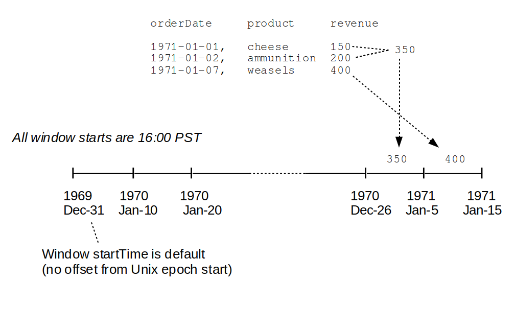
Note that the first reporting window in our output begins on 1970-12-26 16:00:00, even though all of our forecasts are for dates in 1971. Most end users would probably be confused by this. Why should a report for a batch of events projected for 1971 start in 1970, and with a start time at 4pm each day? A more sensible window start would be midnight on the first of the month (January, 1971), rather than towards the end of the last month of the prior year at some time in the afternoon. Why did Spark give us this result?
The answer to this question can be found in in the documentation for the fourth argument to the Spark SQL window function. This argument, startTime is:
the offset with respect to 1970-01-01 00:00:00 UTC with which to start window intervals. For example, in order to have hourly tumbling windows that start 15 minutes past the hour, e.g. 12:15-13:15, 13:15-14:15… provide
startTimeas15 minutes.
Let’s look at the implications of this. Conceptually, Spark sets itself up to organize aggregated data into windows which start at time zero of the Unix epoch. At T-0 our local clocks in the PST time zone (eight hours behind UTC) would have read 4 PM (16:00), and the date would have been Dec 29th. So our first available window starts at this date and time. Since our window interval is 10 days, the start and end time of each subsequent window can be calculated by adding 10 days to the start and end times of the previous window. The diagram below illustrates this. If you were to manually calculate the series of 10 day windows periods beginning at Unix epoch start and ranging to the first few days in 1971 you would eventually ‘generate’ a window with a start time of 4 PM, Dec 26 1970.
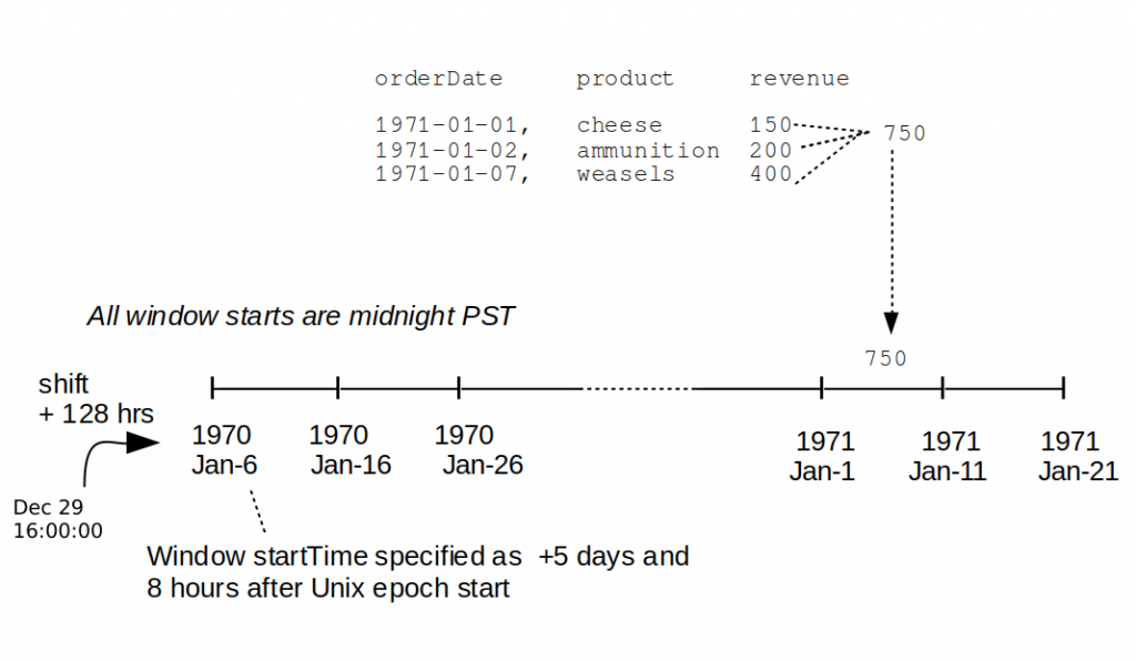
So let us try to shift startTime (using the fourth argument to window) to account for time zone difference. We need to add 8 hours to account for the time zone difference. That would bump the time of the first window that ‘buckets’ our aggregated data to December 27th 1970, but that is still 5 days prior to our desired first window start date of midnight January 1, 1971. So we specify a startTime offset of 5 * 24(hours) + 8(hours) = 128 hours, by passing the string “128” to our revenueReport method. Then we get the expected result as shown below.
revenueReport("128")
// RESULT:
// +------------------------------------------+-----------------+
// |period                                    |sum(projectedRev)|
// +------------------------------------------+-----------------+
// |[1971-01-01 00:00:00, 1971-01-11 00:00:00]|750              |
// +------------------------------------------+-----------------+
The effect of the + 128 hour shift on the start times of our windows can be shown graphically:
So, if we are in time zone PST, should we always specify our startTime offset as 128? Clearly not, since the number of days by which we need to shift will be affected by factors such as variance in the number of days in each month, and leap years. But it would certainly be handy to have a method for automatically calculating the appropriate shift interval for any given data set.
Below is a first-cut prototype of such a method. It is not production ready. For example, it only handles intervals in units of days, but it should give you an idea of how to automate the general problem of finding the appropriate shift amount. It works for cases where the time stamps on to-be-processed data are all after Unix epoch start, and where window intervals are in days.
  /**
    * Return the offset in hours between the default start time for windowing
    * operations (which is Unix epoch start at UTC), and the desired start time
    * of the first window to output for our data set.
    *
    * The desired start time of the first window  is assumed to be midnight of the first
    * day of the month _not_later_than_ the earliest time stamp in the dataframe 'df'.
    *
    * This is a proof of concept method. It will only work if the earliest time stamp
    * in the input data set occurs after Unix epoch start. The window and slide interval are
    * assumed to be identical, with both in units of days.
    *
    * @param df           - input data frame
    * @param timeStampCol - which column to treat as timestamp
    * @param windowLenDays - length of grouping window to be applied (in days)
    * @return integer value of offset in hours via which start window should be shifted, this value
    *         should be passed as the fourth argument to the Spark SQL window function (the startTime).
    */
  import org.apache.spark.sql.DataFrame
  def hoursOffsetToFirstWindow(df: DataFrame,
                               timeStampCol: String,
                               windowLenDays: Integer): Long = {
    import java.time.{Instant, LocalDateTime, Duration, ZoneId}

    val ets: LocalDateTime =    // earliest timestamp in dataframe
      df.orderBy(timeStampCol).first().
        getAs[java.sql.Timestamp](timeStampCol).toLocalDateTime
    val firstDayOfWindow: LocalDateTime =
      LocalDateTime.of(ets.getYear, ets.getMonthValue, 1, 0, 0)
    val epochStartUtc =
      LocalDateTime.ofInstant(Instant.ofEpochSecond(0), ZoneId.systemDefault())
    val hoursPerWindowPeriod =
      windowLenDays * 24
    val hoursDiff =
      Duration.between(epochStartUtc, firstDayOfWindow).toHours
    hoursDiff % hoursPerWindowPeriod
  }
The method takes in a dataframe and the name of the column that holds the time stamp information. It grabs the earliest time frame in the data frame as ets, and uses that variable to find firstDayOfWindow (the maximally valued first day of the month not occurring after the earliest time stamp in the dataframe), relative to local time. The method then gets the start of the Unix epoch (epochStartUtc) as a LocaleDateTIme and computes the difference between epochStartUtc and firstDayOfWindow. It returns that difference modulo the number of hours in the window period for the aggregation to be performed. One general principle to note from this method is that when computing the difference between two times it is useful to convert both the to-be-compared times to LocaleDateTime.
When we invoke our prototype method like this:
hoursOffsetToFirstWindow(input, "timestamp", 10)
// Result:  res7: Long = 128
the result is the correct value by which we need to shift startTime: 128 hours.
Conclusion
Dealing with time in Spark (and Scala/Java in general) can be really confusing. In this article we’ve done our best to present techniques and information that will lessen some of that confusion. If you take away only one thing after your initial read, our recommendation is that you remember that when rendering time stamps the observed String values will vary depending on your local time zone. But you can always get a better idea of what is going on internally by casting your time stamp to “integer”. Time to wrap up.