Author Archives: chris

Integration Test Support and Reconfiguration of the ‘Test’ Task via Gradle Plug-in. (WORK IN PROGRESS !)

Introduction

Our amazing Internet abounds with useful guidelines on what to put in our unit tests and what should go in integration tests. So rather than recapping those discussions, I will begin this post by simply noting that in our builds we usually want to have the option of running these independently of one another. We typically want our unit tests to run fairly quickly without requiring external set-up (e.g., launching a database instance, connecting to a VPN, etc.), while we are fine with imposing those requirements on our integration tests. This is because the module which is being integrated with ‘something else’ will have dependencies on that ‘something else’, and launching or connecting to a test instance of the ‘something else’ may slow down your ‘code, test, debug’ development cycle. Many developers prefer to run only unit tests in the ‘test’ phase of that cycle, and defer running integration tests until they are ready to push their latest commits to a shared code repository

The test framework I tend to use, testNG, has support for separating out unit tests from integration tests. However, we need to do some extra work in our build.gradle files to set up a task that allows us to run the latter. Doing this over and over for every project can be a pain. Fortunately, Gradle’s plug-in mechanism provides an easy way for you to share a re-useable plug-in module which does such set-up, eliminating the need for others in your organization to continually copy/paste mystery code snippets of code. The goal of this post is to explain the workings of the simple Gradle plug-in I wrote to accomplish this task (not 100% perfect yet, see Caveats section), and to show you how such plug-ins can be published to a a Maven repository. Such publication enables your test configuration to be shared with any future project via one additional line in that project’s build.gradle file.

Some reasons why this article might be more useful than the many ‘Hello World’ plug-in tutorials out there: the plug-in code we will walk through not only adds a new Gradle task (integrationTest), it also re-configures an existing task. This type of customization turned out to be quite difficult (at least for me), and I came up dry in my search for supporting examples and/or tutorials on this particular aspect of Gradle plug-in-ology. Neither was I able to find any article that walked me through publishing and consuming my plug-in to/from a Maven repo, so the how-to I provide on that might also be of some unique value.

A final prefatory note: the commands I list for you to follow along with will work with MacOS and Linux, and possibly if you are on Windows using the Cygwin shell. If you don’t have any of those three then you’ll have to tinker to run the examples. I also use Scala in the examples, so if you are Java-only, you’ll have to use your imagination (sorry). Oh, and you’ll also need Docker for the publish part. I could have used the raw file system as a Maven repo, but I happened to be using Nexus running under Docker, and am too lazy to change for the sake of this article.

The Simplest (non-reuseable) Way of Setting up Integration Test Support

Let’s set up integration test support manually first, without a plug-in. The following command sequence should work to setup a simple ‘canned’ project (using Gradle 7.x — might work for other versions, but no guarantees):

dir=/tmp/catbox ; rm -rf $dir ; mkdir $dir ;  cd $dir 
gradle init --type scala-application 

In response to the prompts, type:

1<RETURN>
<RETURN>
<RETURN>

And you should see output like this:

To be sure all is well, run the command ‘gradlew build’ and make sure you see ‘BUILD SUCCESSFUL’ as output. After that’s all working, let’s add a TestNG test, like this:

cat < app/src/test/scala/UnitTest.scala
import org.testng.annotations.Test
class UnitTest {
@Test def test(): Unit = {
if ( "true" == System.getenv("testShouldFail") ) {
assert(2> 10)
} else {
assert(2> 1)
}
}
}
EOF

And next we will try to run it, setting the environment variable that will force the test to fail. We type:

( export testShouldFail=true ; gradlew 'app:test' )

But we note that we see output indicating BUILD SUCCESSFUL. Did our tests even run? Spoiler: it didn’t even compile . This is because out-of-the-box gradle builds expect you to write tests using Junit, not TestNG. To correct that we will change our configuration to use TestNG’s test runner, by adding the the Gradle configuration code below. Note that we are eventually going to make use of TestNG’s support for using annotations to group related sets of tests https://testng.org/doc/documentation-main.html#test-groups. We will configure the test task to not run tests annotated to be in the integrationTest group. Those tests will only run if we invoke the ‘integrationTest’ task, which we will add in the next step. For now, type the following:

cat <> app/build.gradle
test {
useTestNG() { // this switches framework from Junit to TestNG
excludeGroups "integrationTest"
useDefaultListeners = true
}
}
EOF

Next, add a dependency on TestNG, if you are on a platform that supports shell, then this command sequence should do it:

cat   app/build.gradle  | \
    sed -e 's/dependencies.*{/dependencies {  testImplementation group: "org.testng", name: "testng", version: "6.8"/' > tmp

mv tmp app/build.gradle  

If that doesn’t work, add in the dependency manually. After ‘dependencies {‘ in app/build.gradle, add:

testImplementation group: "org.testng", name: "testng", version: "6.8"

If you try running the previous command sequence again you should see a test failure rather than compilation errors:

( export testShouldFail=true ; gradlew 'app:test' )

And if we don’t force failure by setting the environment variable, that is, if we simply run

  gradlew 'app:test' 

and then we should see ‘BUILD SUCCESSFUL’ in our output. Now we are in good shape to try to add integration tests and run them separately. Add the test as follows:

cat < app/src/test/scala/IntegrationTest.scala
import org.testng.annotations.Test
class IntegrationTest {
@Test(groups = Array("integrationTest")) def test(): Unit = {
if ( "true" == System.getenv("integrationTestShouldFail") ) {
assert(2> 10)
} else {
assert(2> 1)
}
}
}
EOF

Does the test fail when we run the ‘test’ task? Try it.

    ( export integrationTestShouldFail=true ; gradlew 'app:test' )

Well we explicitly excluded tests annotated as ‘integrationTest’, so that’s why nothing ran.
To remedy this let’s add a specialized task to our build config to run only these such tests.

cat <> app/build.gradle
task integrationTest(type: Test) {
useTestNG() {
includeGroups 'integrationTest'
}
}
EOF

And now invoke the new test target we just added and see if it now fails:

 ( export integrationTestShouldFail=true ; gradlew 'app:integrationTest' )

If all went well the run should result in an assertion failure with the message “IntegrationTest.test FAILED”


From Copy/Paste Re-Use to Plug-ins

The modifcations to build.gradle that we made above were not hugely complex or time-consuming, but they were still necessary to introduce a relatively minor customization to Gradle’s out-of-the-box behavior. Clearly the more customizations you add in this way the more the possibility for mistakes creeps in. If you want to enforce the use of TestNG and unit test / integration test separation as organizational standards you don’t want this config copy/pasted accross numerous projects. It obscures the build logic that is particular to the project, and it makes upgrades and changes much harder. So let’s implement the above as a plug-in, such that the desired configuration can be set using one line of Gradle configuration code.

Publishing and Consuming the Plug-in via Nexus (running in Docker)

Missing from many plug-in tutorials are examples of how to publish the plug-in for consumption (re-use) in other projects. We will demonstrate that here using Nexus, a Maven repository manager. This could also be done with Artifactory or other products, but I will use Nexus here. I won’t go into details on use of Docker. But, I will guarantee: if you are not using it now, you are missing out. Assuming you have Docker installed, Nexus can be launched via this one-liner

    docker run -d -p 8081:8081 --name nexus sonatype/nexus:oss

Type this URL in your browser to bring up the UI:

     http://localhost:8081/nexus/

It might take 10 seconds or so, and you might have to refresh a couple of times. You should eventually see a screen like this.

OKAY …. need to write part about how to do what we did above manually and show code for plugin.. Code for plugin lives here-> https://github.com/buildlackey/gradle-test-configuration-plugin

Unit & Integration Testing Kafka and Spark

Overview

Kafka is one of the most popular sources for ingesting continuously arriving data into Spark Structured Streaming apps. However, writing useful tests that verify your Spark/Kafka-based application logic is complicated by the Apache Kafka project’s current lack of a public testing API (although such API might be ‘coming soon’, as described here).

This post describes two approaches for working around this deficiency and discusses their pros and cons. We first look at bringing up a locally running Kafka broker in a Docker container, via the helpful gradle-docker-compose plug-in. (Side note: although our examples use Gradle to build and run tests, translation to Maven “should be” (TM) straightforward.) This part of the article assumes basic knowledge of Docker and docker-compose. Next we look at some third party (i.e., unaffiliated with Apache Kafka) libraries which enable us to run our tests against an in-memory Kafka broker. In the last section we will look at some of the upgrade issues that might arise with the embedded / in-memory Kafka broker approach when we migrate from older to newer versions of Spark. To start off, we’ll walk you through building and running the sample project.

Building and Running the Sample Project

Assuming you have Docker, docker-compose, git and Java 1.8+ installed on your machine, and assuming you are not running anything locally on the standard ports for Zookeeper (2181) and Kafka (9092), you should be able to run our example project by doing the following:

git clone git@github.com:buildlackey/kafka-spark-testing.git
cd kafka-spark-testing
git checkout first-article-spark-2.4.1
gradlew clean test integrationTest

Next, you should see something like the following (abbreviated) output:

> Task :composeUp
    ...
Creating bb5feece1xxx-spark-testing__zookeeper_1 ...
    ...
Creating spark-master               ...
    ...
Creating spark-worker-1             ... done
    ...
Will use 172.22.0.1 (network bb5f-xxx-spark-testing__default) as host of kafka
    ...
TCP socket on 172.22.0.1:8081 of service 'spark-worker-1' is ready
    ...
+----------------+----------------+-----------------+
| Name           | Container Port | Mapping         |
+----------------+----------------+-----------------+
| zookeeper_1    | 2181           | 172.22.0.1:2181 |
+----------------+----------------+-----------------+
| kafka_1        | 9092           | 172.22.0.1:9092 |
+----------------+----------------+-----------------+
| spark-master   | 7077           | 172.22.0.1:7077 |
| spark-master   | 8080           | 172.22.0.1:8080 |
+----------------+----------------+-----------------+
| spark-worker-1 | 8081           | 172.22.0.1:8081 |
+----------------+----------------+-----------------+

    ...

BUILD SUCCESSFUL in 39s
9 actionable tasks: 9 executed

Note the table showing names and port mappings of the locally running containers brought up by the test. The third column shows how each service can be accessed from your local machine (and, as you might guess, the IP address will likely be different when you run through the set-up).

Testing Against Dockerized Kafka

Before we get into the details of how our sample project runs tests against Dockerized Kafa broker instances, let’s look at the advantages of this approach over using in-memory (embedded) brokers.

  • Post-test forensic analysis. One advantage of the Docker-based testing approach is the ability to perform post-test inspections on your locally running Kafka instance, looking at things such as the topics you created, their partition state, content, and so on. This helps you answer questions like: “was my topic created at all?”, “what are its contents after my test run?”, etc.
  • Easily use same Kafka as production. For projects whose production deployment environments run Kafka in Docker containers this approach enables you to synchronize the Docker version you use in tests with what runs in your production environment via a relatively easy configuration-based change of the Zookeeper and Docker versions in your docker-compose file.
  • No dependency hell. Due to the absence of ‘official’ test fixture APIs from the Apache Kafka project, if you choose the embedded approach to testing, you need to either (a) write your own test fixture code against internal APIs which are complicated and which may be dropped in future Kafka releases, or (b) introduce a dependency on a third party test library which could force you into ‘dependency hell’ as a result of that library’s transitive dependencies on artifacts whose versions conflict with dependencies brought in by Spark, Kafka, or other key third party components you are building on. In the last section of this post, we will relive the torment I suffered in getting the embedded testing approach working in a recent client project.

Dockerized Testing — Forensic Analysis On Running Containers

Let’s see how to perform forensic inspections using out of-the-box Kafka command line tools. Immediately after you get the sample project tests running (while the containers are up), just run the following commands. (These were tested on Linux, and “should work” (TM) on MacOS):

mkdir /tmp/kafka
cd /tmp/kafka
curl https://downloads.apache.org/kafka/2.2.2/kafka_2.12-2.2.2.tgz  -o /tmp/kafka/kafka.tgz
tar -xvzf kafka.tgz  --strip 1
export PATH="/tmp/kafka/bin:$PATH"
kafka-topics.sh  --zookeeper localhost:2181   --list

You should see output similar to the following:

__consumer_offsets
some-testTopic-1600734468638

__consumer_offsets is a Kafka system topic used to store information about committed offsets for each topic/partition, for each consumer group. The next topic listed — something like some-testTopic-xxx — is the one created by our test. It contains the content: ‘Hello, world’. This can be verified by running the following command to see what our test wrote out to the topic:

kafka-console-consumer.sh    --bootstrap-server localhost:9092   \
                 --from-beginning  --topic some-testTopic-1600734468638

The utility should print “Hello, world”, and then suspend as it waits for more input to arrive on the monitored topic. Press ^C to kill the utility.


Dockerized Testing — Build Scaffolding

In the listing below we have highlighted the key snippets of Gradle configuration that ensure Docker and ZooKeeper containers have been spun up before each test run. Lines 1-4 simply declare the plug-in to activate. Line 7 ensures that when we run the integrationTest task the dockerCompose task will be executed as a prerequisite to ensure required containers are launched. Since integration tests — especially those that require Docker images to be launched, and potentially downloaded — typically run longer than unit tests, our build script creates a custom dependency configuration to run such tests, and makes them available via the separate integrationTest target (to be discussed more a little further on), as distinct from the typical way to launch tests: gradlew test.

Lines 10 – 17 configure docker-compose’s behavior, with line 10 indicating the path to the configuration file that identifies the container images to spin up, environment variables for each, the order of launch, etc. Line 13 references the configuration attribute that ensures containers are left running. The removeXXX switches that follow are set to false, but if you find that Docker cruft is eating up a lot of your disk space you might wish to experiment with settings these to true.

plugins {
  ...
  id "com.avast.gradle.docker-compose" version "0.13.3"
}


dockerCompose.isRequiredBy(integrationTest)

dockerCompose {
  useComposeFiles = ["src/test/resources/docker-compose.yml"]

  // We leave containers up in case we want to do forensic analysis on results of tests
  stopContainers = false
  removeContainers = false  // default is true
  removeImages = "None"     // Other accepted values are: "All" and "Local"
  removeVolumes = false     // default is true
  removeOrphans = false     // removes contain
}

The Kafka-related portion of our docker-compose file is reproduced below, mainly to highlight the ease of upgrading your test version of Kafka to align with what your production team is using — assuming that your Kafka infrastructure is deployed into a Docker friendly environment such as Kubernetes. If your prod team deploys on something like bare metal this section will not apply. But if you are lucky, your prod team will simply give you the names and versions of the Zookeeper and Kafka images used in your production deployment. You would replace lines 4 and 8 with those version qualified image names, and as your prod team deploys new versions of Kafka (or Zookeeper) you simply have those two lines to change to stay in sync. This is much easier than fiddling with versions of test library .jar’s due to the attendant dependency clashes that may result from such fiddling. Once the Kafka project releases an officially supported test kit this advantage will be less compelling.

version: '2'
 services:
   zookeeper:
     image: wurstmeister/zookeeper:3.4.6
     ports:
       - "2181:2181"
   kafka:
     image: wurstmeister/kafka:2.13-2.6.0
     command: [start-kafka.sh]
     ports:
       - "9092:9092"
     environment:
       KAFKA_ZOOKEEPER_CONNECT: zookeeper:2181
       KAFKA_ADVERTISED_HOST_NAME: 127.0.0.1
     volumes:
       - /var/run/docker.sock:/var/run/docker.sock
     depends_on:
       - zookeeper


Dockerized Testing — Build Scaffolding: Running Integration Tests Separately

The listing below highlights the portions of our project’s build.gradle file which enable our integration test code to be stored separately from code for our unit tests, and which enable the integration tests themselves to be run separately.

sourceSets {
  integrationTest {
    java {
      compileClasspath += main.output + test.output
      runtimeClasspath += main.output + test.output
      srcDir file("src/integration-test/java")
    }
    resources.srcDirs "src/integration-test/resources", "src/test/resources"
  }
}

configurations {
  integrationTestCompile.extendsFrom testCompile
}


task integrationTest(type: Test) {
  testClassesDirs = sourceSets.integrationTest.output.classesDirs
  classpath = sourceSets.integrationTest.runtimeClasspath
}

integrationTest {
  useTestNG() { useDefaultListeners = true }
}

dockerCompose.isRequiredBy(integrationTest)

Lines 1-10 describe the integrationTest ‘source set’. Source sets are logical groups of related Java (or Scala, Kotlin, etc.) source and resource files. Each logical group typically has its own sets of file dependencies and classpaths (for compilation and runtime). Line 6 indicates the top level directory where integration test code is stored. Line 8 identifies the locations of directories which hold resources to be made available to the runtime class path. Note that we specify both src/test/resources (as well as src/integrationTest/resources) so any configuration we put under the former directory is also available to integration tests at runtime. This is useful for things like logger configuration, which is typically the same for both types of tests, and as a result is a good candiate for sharing.

Line 12 defines the ‘custom dependency configurationintegrationTest. A dependency configuration in Gradle is similar to a Maven scope — it maps roughly to some build time activity which may require distinct dependencies on specific artifacts to run. Line 13 simply states that that the integrationTest dependency configuration should inherit its compile
path from the testCompile dependency configuration which is available out-of-the box via the java plugin. If we wanted to add additional dependencies — say on guava — just for our integration tests, we could do so by adding lines like the ones below to the ‘dependencies’ configuration block:

dependencies {
integrationTestCompile group: 'com.google.guava', name: 'guava', version: '11.0.2'
…. // other dependenacies
}

Line 17 – 20 define ‘integrationTest’ as an enhanced custom task of type Test. Tests need a
test runner, which for Gradle is junit by default. Our project uses testNG, so we declare this on line 23. (Side note: line 4 seems to state the same thing as line 13, but I found both were required for compilation to succeed).

We didn’t touch on code so much in this discussion, but as you will see in the next section the test code that runs against Dockerized Kafka brokers shares many commonalities with the code we wrote to test against embedded brokers. After reading through the next section you should be able to understand what is going on in ContainerizedKafkaSinkTest.

Embedded Broker Based Testing

We described some of the advantages of Docker-based testing of Kafka/Spark applications in the sections above, but there are also reasons to prefer the embedded approach:

  • Lowered build complexity (no need for separate integration tests and docker-compose plug-in setup).
  • Somewhat faster time to run tests, especially when setting up a new environment, as there is no requirement to downloaded images.
  • Reduced complexity in getting code coverage metrics if all your tests are run as unit tests, within the same run. (Note that if this were a complete no-brainer then there would be not be tons of how-to articles out there like this.)
  • Your organization’s build infrastructure might not yet support Docker (for example, some companies might block downloads of images from the “Docker hub” site).

So, now let’s consider how to actually go about testing against an embedded Kafka broker. First, we need to choose a third-party library to ease the task of launching said broker . I considered several, with the Kafka Unit Testing project being my second choice, and Spring Kafka Test ending up as my top pick. My main reasoning was that the latter project, being backed by VMware’s Spring team is likely to work well into the future, even as the Kafka internal APIs it is based on may change. Also, the top level module for spring-kafka-test only brought in about six other Spring dependencies (beans, core, retry, aop, and some others), rather than the kitchen sink, as some might fear.

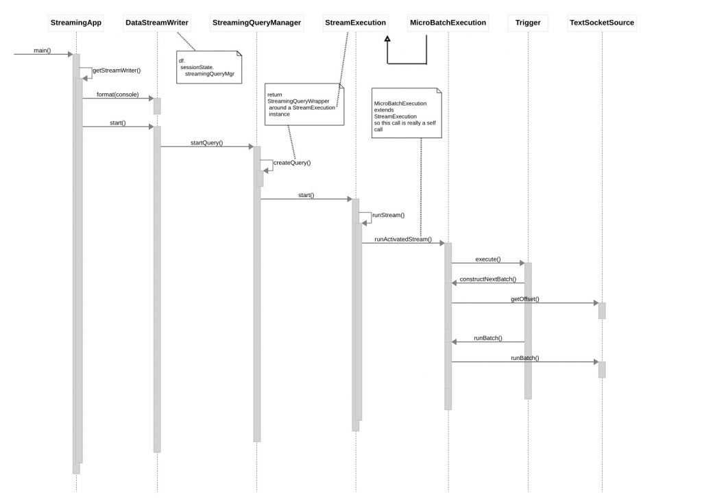
With our test library now chosen let’s look at the code, the overall organization of which we present diagrammatically:

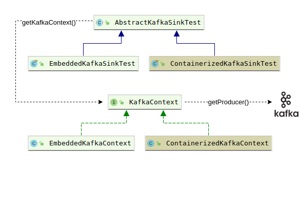
Our KafkaContext interface declares the getProducer() method to get at a Kafka producer which is used simply to send the message ‘Hello, world’ to a topic (lines 18-20 of the listing for AbstractKafkaSinkTest shown below). Our abstract test class then creates a Dataset of rows that return the single key/value pair available from our previous write to the topic (lines 23-28), and finally checks that our single row Dataset has the expected content (lines 32-37).

public abstract class AbstractKafkaSinkTest {
  final Logger logger = LoggerFactory.getLogger(AbstractKafkaSinkTest.class);

  protected static final String topic = "some-testTopic-" + new Date().getTime();
  protected static final int kafkaBrokerListenPort = 6666;

  KafkaContext kafkaCtx;

  abstract KafkaContext getKafkaContext() throws ExecutionException, InterruptedException;

  @BeforeTest
  public void setup() throws Exception {
    kafkaCtx = getKafkaContext();
    Thread.sleep(1000);           // TODO - try reducing time, or eliminating
  }

  public void testSparkReadingFromKafkaTopic() throws Exception {
    KafkaProducer<String, String> producer =  kafkaCtx.getProducer();
    ProducerRecord<String, String> producerRecord = new ProducerRecord<String, String>(topic, "dummy", "Hello, world");
    producer.send(producerRecord);

    SparkSession session = startNewSession();
    Dataset<Row> rows = session.read()
      .format("kafka")
      .option("kafka.bootstrap.servers", "localhost:" + kafkaCtx.getBrokerListenPort())
      .option("subscribe", topic)
      .option("startingOffsets", "earliest")
      .load();

    rows.printSchema();

    List<Row> rowList = rows.collectAsList();
    Row row = rowList.get(0);
    String strKey = new String(row.getAs("key"), "UTF-8");
    String strValue = new String(row.getAs("value"), "UTF-8");
    assert(strKey.equals("dummy"));
    assert(strValue.equals("Hello, world"));
  }

  SparkSession startNewSession() {
    SparkSession session = SparkSession.builder().appName("test").master("local[*]").getOrCreate();
    session.sqlContext().setConf("spark.sql.shuffle.partitions", "1");   // cuts a few seconds off execution time
    return session;
  }
}

AbstractKafkaSinkTest delegates to its subclasses the decision of what kind of context (embedded or containerized) will be returned from getKafkaContext() (line 9, above). EmbeddedKafkaSinkTest, for example, offers up an EmbeddedKafkaContext, as shown on line 3 of the listing below.

public class EmbeddedKafkaSinkTest extends AbstractKafkaSinkTest {
  KafkaContext getKafkaContext() throws ExecutionException, InterruptedException {
    return new EmbeddedKafkaContext(topic, kafkaBrokerListenPort);
  }

  @Test
  public void testSparkReadingFromKafkaTopic() throws Exception {
    super.testSparkReadingFromKafkaTopic();
  }
}

The most interesting thing about EmbeddedKafkaContext is how it makes use of the EmbeddedKafkaBroker class provided by spring-kafka-test. The associated action happens on lines 10-15 of the listing below. Note that we log the current run’s connect strings for both Zookeeper and Kafka. The reason for this is that — with a bit of extra fiddling — it actually is possible to use Kafka command line tools to inspect the Kafka topics you are reading/writing in your tests. You would need to introduce a long running (or infinite) loop at the end of your test that continually sleeps for some interval then wakes up. This will ensure that the Kafka broker instantiated by your test remains available for ad hoc querying.

public class EmbeddedKafkaContext implements KafkaContext {
  final Logger logger = LoggerFactory.getLogger(EmbeddedKafkaContext.class);
  private final int kafkaBrokerListenPort;
  private final String bootStrapServers;
  private final String zookeeperConnectionString;

  EmbeddedKafkaContext(String topic, int kafkaBrokerListenPort) {
    this.kafkaBrokerListenPort =  kafkaBrokerListenPort;

    EmbeddedKafkaBroker broker = new EmbeddedKafkaBroker(1, false, topic);
    broker.kafkaPorts(kafkaBrokerListenPort);
    broker.afterPropertiesSet();
    zookeeperConnectionString = broker.getZookeeperConnectionString();
    bootStrapServers = broker.getBrokersAsString();
    logger.info("zookeeper: {}, bootstrapServers: {}", zookeeperConnectionString, bootStrapServers);
  }

  @Override
  public int getBrokerListenPort() {
    return kafkaBrokerListenPort;
  }
}

public class EmbeddedKafkaSinkTest extends AbstractKafkaSinkTest {
  KafkaContext getKafkaContext() throws ExecutionException, InterruptedException {
    return new EmbeddedKafkaContext(topic, kafkaBrokerListenPort);
  }

  @Test
  public void testSparkReadingFromKafkaTopic() throws Exception {
    super.testSparkReadingFromKafkaTopic();
  }
}


Embedded Broker Based Testing Downsides: Dependency Hell

We mentioned earlier that one upside of Dockerized testing is the ability to avoid dependency conflicts that otherwise could arise as a result of bringing in a new test library, or upgrading Spark (or other third party components) after you finally manage to get things to work. If you pull the sample project code and execute the command git checkout first-article-spark-2.4.1 you will see that for this version of Spark we used an earlier version of spring-kafka-test (2.2.7.RELEASE versus 2.4.4.RELEASE, which worked for Spark 3.0.1). You should be able to run gradlew clean test integrationTest just fine with this branch in its pristine state. But note the lines at the end of build.gradle in this version of the project:

configurations.all {
  resolutionStrategy {
    force 'com.fasterxml.jackson.core:jackson-databind:2.6.7.1'
  }
}

If you were to remove these lines our tests would fail due to the error “JsonMappingException: Incompatible Jackson version: 2.9.7“. After some digging we found that it was actually spring-kafka-test that brought in version 2.9.7 of jackson-databind, so we had to introduce the above directive to force all versions back down to the version of this dependency used by Spark.

Now after putting those lines back (if you removed them), you might want to experiment with what happens when you upgrade the version of Spark used in this branch to 3.0.1. Try modifying the line spark_version = "2.4.1" to spark_version = "3.0.1" and running gradlew clean test integrationTest again. You will first get the error “Could not find org.apache.spark:spark-sql_2.11:3 0.1.“. That is because Scala version 2.11 was too old for the Spark 3.0.1 team to release their artifacts against. So we need to change the line scala_version = "2.11" to scala_version = "2.12" and try running our tests again.

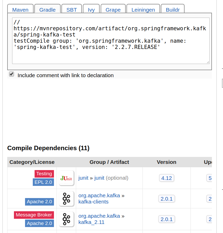
This time we see our tests fail at the very beginning, in the setup phase, with the error “NoSuchMethodError: scala.Predef$.refArrayOps([Ljava/lang/Object;)Lscala/collection/mutable/ArrayOps“. This looks like we might be bringing in conflicting versions of the Scala runtime libraries. Indeed if we look at the dependency report for spring-kafka-test version 2.2.7.RELEASE we see (at the bottom of the page reproduced below) that this version of spring-kafka-test brings in org.apache.kafka:kafka_2.11:2.0.1. This is a version of Kafka that was compiled with Scala 2.11, which results in a runtime clash between that version and the version that Spark needs (2.12). This problem was very tricky to resolve because the fully qualified (group/artifact/version) coordinates of spring-kafka-test:2.2.7.RELEASE offer no hint of this artifact’s dependency on Scala 2.11.

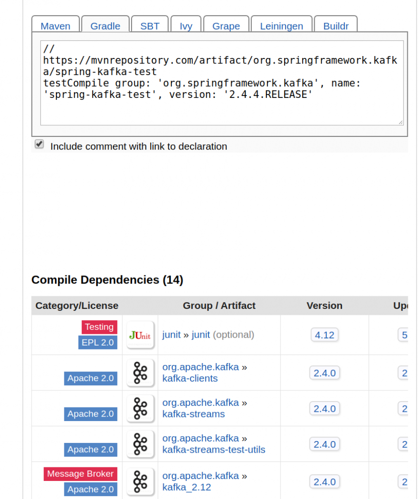
Once I realized there was a Scala version conflict it was a pretty easy decision to hunt around for a version of spring-kafka-test that was compiled against a release of Kafa which was, in turn, compiled against Scala 2.12. I found that in version 2.4.4, whose abbreviated dependency report is shown below.

Hopefully this recap of my dependency-related suffering gives you some motivation to give Docker-based testing a try !

A Tail-recursion-ification Example

This post walks through some of the thinking behind how we might approach the problem of converting a non-tail recursive function to a tail recursive one. The code we present also illustrates some interesting Scala techniques: implicit conversions of primitive classes to Ordered, type aliases and function passing. For those of you not already familiar with tail recursion, there are some great articles out there to get up to speed on the concept (for example, this one).

To summarize very briefly:

  • tail recursion is a characteristic of recursive methods wherein the very last action of any branch of the method is a recursive call to the method itself.
  • recursive functions that are not tail recursive have the annoying property of blowing out your stack because they save intermediate state in each stack frame — state which is then combined by the result of the recursive call. Given that stack memory is finite, and assuming that your input could be arbitrarily long (therefore requiring an arbitrarily large number of stack frames to store intermediate state) you will likely run into a stack overflow at some point.
  • Scala automatically optimizes tail recursive functions by converting the recursion into a loop. This article presents a really good simple example of how tail recursion in the source code is translated to a loop in the byte code.

Now that you are a tail recursion expert, let’s look at some code:

package scalaTry

class Merger[T]()(implicit e: T => Ordered[T]) {
  def compare(a: T, b: T): Unit = {
    if (a < b)
      println("a less")
    else
      println("a NOT less")
  }

  final def merge(a: List[T],
                  b: List[T]): List[T] = {
    (a,b) match{
      case (Nil,Nil) =>
        Nil
      case (a1::tail, Nil) =>
        a1::tail
      case (Nil, b1::tail) =>
        b1::tail
      case (a1::tail1, b1::tail2) =>
        if (a1 < b1) {
          a1::b1::merge(tail1,tail2)
        } else {
          b1::a1::merge(tail1,tail2)
        }
      case default =>
        throw new
            IllegalStateException(
              "Should never get here")
    }
  }

The merge method of the Merger class shown above recursively merges two sorted lists, a and b. The lowest level escape conditions are where one or both of the input lists are empty (Nil). In this case we either return Nil (where both are Nil), or we return the non-Nil list. If both lists are non-Nil, the logic is (conceptually) to create a two element list consisting of the heads of a and b (in their proper order), and append to this two element list the result of merging the tails of a and b (lines 22 and 24).

One interesting aspect of the Merger class, the use of Ordered, and the implicit conversion of T to an Ordered[T] highlighted on line 3, is not specifically related to tail recursion. This line genericizes (in Java-speak) the Merger class such that the merge method can accept Lists of any type T for which an implicit conversion to Ordering is available.

But let’s get back to tail recursion, or the lack of it in the merge method. As discussed above lines 22 and 24 are doing the conceptual equivalent of creating creating a two element list, then recursing on the tails of the input list. The two element list occupies memory on the stack until the recursive call to merge returns, at which point the two element list and the result of the recursive call are joined together. Clearly, more and more memory will be consumed as the input lists get larger.

So what to do? The merge2 function shown below shows one way we can avoid a stack overflow. In this function we explicitly create the list that is to be prepended to the result of merging the tails. But instead of keeping that list on the stack and joining it to the result of the recursive call on the tails, we explicitly pass it down to the recursive call as the prefixSoFar. At the point of each recursive call we know that the elements in prefixSoFar are less than or equal to the head items of either a or b (the variables a1 and b1). Thus when we create a new prefix (as on line 16), we know that prefixSoFar should come first, followed by either a1 then b1, or by b1, then a1 (as on line 20). When one or both of the input lists a and b are Nil, we return the prefixSo far, potentially tacking on any remaining elements in one of the non-Nil input lists (as on line 10). These remaining elements are guaranteed to be equal to or greater than any of the elements of the prefixSoFar (per the given Ordering).

A final comment on the merge2 method: note that Scala provides the handy annotation tailrec, used on line 2, to declare a function as tail recursive, and have the compiler double check that this declaration is correct. If you were to use this annotation right before the method declaration of a non-tail recursive function such as merge, you would get a compiler error.

  def merge2(a: List[T], b: List[T]): List[T] = {
    @scala.annotation.tailrec
    def merge2(a: List[T],
               b: List[T],
               prefixSoFar: List[T]): List[T] = {
      (a,b) match{
        case (Nil,Nil) =>
          prefixSoFar
        case (a1::tail, Nil) =>
          prefixSoFar ::: a1 :: tail
        case (Nil, b1::tail) =>
          prefixSoFar ::: b1 :: tail
        case (a1::tail1, b1::tail2) =>
          if (a1 < b1) {
            val prefix: List[T] =
              prefixSoFar ::: a1 :: b1 :: Nil
            merge2(tail1, tail2, prefix)
          } else {
            val prefix: List[T] =
              prefixSoFar ::: b1 :: a1 :: Nil
            merge2(tail1, tail2, prefix)
          }
        case default =>
          throw new
              IllegalStateException(
                "Should never get here")
      }
    }

    merge2(a, b, Nil)
  }

So, now we have a merge method that won’t blow out our stack. Next we need to test it, which we shall do with the code below. doMergeTest accepts two functions, one that merges two String lists, and another that merges two Int lists. We define the type aliases MergeStringLists and MergeIntLists that capture the signatures of these two functions. doMerge accepts arguments of the first signature as fun1, and the second signature as fun2. In the test ‘merging works’ we first pass in a function pair based on the merge function, and then pass in a function pair based on the tail recursive merge2 function. If you grab the project from this github repo and run it, my guess is that you would see all green. Try it out!

@RunWith(classOf[JUnitRunner])
class MergeTest extends AnyFunSuite {

  type MergeStringLists = (List[String], List[String]) => List[String]
  type MergeIntLists = (List[Int], List[Int]) => List[Int]

  def doMergeTest (fun1: MergeStringLists,
                   fun2: MergeIntLists): Unit = {
    var res = fun1(List[String](), List[String]())
    assert(res.equals(List[String]()))

    res = fun1(List[String](), "foo" :: List[String]())
    assert(res.equals(List[String]("foo")))


    var res2: List[Int] = fun2(2 :: List[Int](), 5 :: List[Int]())
    assert(res2.equals(List[Int](2, 5)))

    res2 = fun2(5 :: Nil, 2 :: Nil)
    assert(res2.equals(List[Int](2, 5)))

    res2 = fun2(5 :: 6 :: Nil, 6 :: Nil)
    assert(res2.equals(List[Int](5, 6, 6)))

    res2 = fun2(6 :: Nil, 5 :: 6 :: Nil)
    assert(res2.equals(List[Int](5, 6, 6)))


    res2 = fun2(5 :: 6 :: Nil, 4 :: 6 :: Nil)
    assert(res2.equals(List[Int](4, 5, 6, 6)))

    res2 = fun2(3 :: 6 :: Nil, 5 :: 6 :: Nil)
    assert(res2.equals(List[Int](3, 5, 6, 6)))
    ()
  }

  test("merging works") {
    val fun1: MergeStringLists =
      (list1: List[String], list2: List[String]) =>
        new Merger[String]().merge(list1, list2)
    val fun2: MergeIntLists =
      (list1: List[Int], list2: List[Int]) =>
        new Merger[Int]().merge(list1, list2)
    doMergeTest(fun1, fun2)

    val fun3: MergeStringLists =
      (list1: List[String], list2: List[String]) =>
        new Merger[String]().merge2(list1, list2)
    val fun4: MergeIntLists =
      (list1: List[Int], list2: List[Int]) =>
        new Merger[Int]().merge2(list1, list2)
    doMergeTest(fun3, fun4)
  }
}

Time Travails With Java, Scala and Apache Spark

Processing data with date/time attributes means having to deal with complicated issues such as leap years, time zones and daylight savings time. Fortunately, for Spark developers, Java (upon which Scala, and therefore Spark, is built) has libraries that help abstract away some of these complexities. And Spark itself has a number of date/time processing related functions, some of which will be explored in this article. We’ll begin with a discussion of time-related pitfalls associated with daylight savings time and programming for audiences in different Locales. We will then examine how the JVM represents time in “Unix epoch format“, and review Spark’s support for ingesting and outputting date strings formatted per the ISO 8601 standard. We will conclude by explaining how to correct the oddly time-shifted output you might encounter when programming windowed aggregations.

Some tricky aspects of dealing with time

Let’s consider the meaning of this time stamp: 2019-03-10 02:00:00. In the US “03-10” would be interpreted as March 10th. In France this string would be understood as October 3rd, since European date formats assume month follows day. Even in the US the interpretation would vary based on the time zone you are in (2 AM in New York occurs three hours ahead of 2 AM in California), and whether or not daylight savings time (DST) is in effect. And trickier still, the observance of DST may not be a given over the years in some states. As of this writing in California there is pending legislation to make daylight savings time permanent (that is to eliminate the ‘fall back’ from ‘Spring forward, fall back’).

If you run the code snippet below you can directly see some of DST’s strange effects. Any timestamp from 2 AM to 3 AM (exclusive) on March 10th 2019 could never be a valid one in the PST time zone, since at 2 AM on that date the clock advanced one hour directly to 3 AM. But in other time zones, such as Asia/Tokyo, this jump would not have occurred.

import java.util.TimeZone


def updateTimeZone(zone: String)  = {
    System.setProperty("user.timezone", zone);
    TimeZone.setDefault(TimeZone.getTimeZone(zone))
} 

// Set timezone to Pacific Standard, where -- at least for now --
// daylight savings is in effect 
updateTimeZone("PST")

java.sql.Timestamp.valueOf("2019-03-10 01:00:00")
// should result in:  java.sql.Timestamp = 2019-03-10 01:00:00.0
    
 java.sql.Timestamp.valueOf("2019-03-09 02:00:00")              // 2 AM
// should result in:  java.sql.Timestamp = 2019-03-09 02:00:00.0

 java.sql.Timestamp.valueOf("2019-03-10 02:00:00")
// should result in:  java.sql.Timestamp = 2019-03-10 03:00:00.0   - 3 AM, not 2 AM as per input !


// Let's now move to Japan time, where day light savings rules are not followed  
updateTimeZone("Asia/Tokyo")

java.sql.Timestamp.valueOf("2019-03-10 01:00:00")
// should result in:  java.sql.Timestamp = 2019-03-10 01:00:00.0

 java.sql.Timestamp.valueOf("2019-03-09 02:00:00")              // 2 AM
// should result in:  java.sql.Timestamp = 2019-03-09 02:00:00.0

 java.sql.Timestamp.valueOf("2019-03-10 02:00:00")
// should result in:  java.sql.Timestamp = 2019-03-10 02:00:00.0   - Doesn't skip 1 hour to 3 AM !

Time and its Java Representations

So dealing with time can be tricky. But as mentioned at the outset, Java libraries abstract away a lot of this complexity. Java represents time in a format called “Unix time” — where ‘time zero’ (T-0) is defined as the instant in time at which the clock struck midnight in the city of Greenwhich England on January 1, 1970. Because of the Greenwhich point of reference the longitudinal zone that subsumes this city is referred to as “GMT” (Greenwhich Mean Time). Another synonym for this time zone is UTC (for Universal Coordinated Time). In Unix time, any instant on the time line before or after T-0 is represented as the number of seconds by which that instant preceded or followed T-0. Any instant prior to T-0 is represented as a negative number, and any subsequent instant is represented as a positive number. (Side note: some classes in Java — like java.util.Date — represent time in terms of milliseconds offset from T-0, other classes might use nanoseconds, but it is always from the same point of reference. For simplicity we’ll mostly frame our discussion in terms of seconds.)

Since Unix time uses only a scalar integer value, with no notion of time zone, a Unix time value cannot be sensibly rendered to a human being in a given region of the world without also specifying that region’s time zone. The result of such rendering would be a time zone-free string like this: 2019-10-11 22:00:00, with the attendant ambiguities discussed earlier.

Time as represented internally in Spark

Spark has various internal classes that represent time. Spark’s internal TimestampType represents time as nanoseconds from the Unix epoch. When accessed by Java or Scala code, internal TimestampType values are mapped to instances of java.sql.Timestamp, which also permits representation of time to nanosecond precision. However there have been some bugs related to being able to parse date/time strings with nanosecond components. But how often do you even need that? At least we can prove that Spark can handle parsing dates to millisecond precision, as shown by the code snippet below. To simplify our discussion this is the last time we will mention or deal with fractions of a second in our timestamps.

List("1970-01-01T00:00:00.123+00:00").toDF("timestr").
          withColumn("ts", col("timestr").cast("timestamp")).
          withColumn("justTheMillisecs", date_format($"ts", "'milliseconds='SSS")).
          drop("timestr").
          drop("ts").
          show(false)
 //RESULT:
 //+----------------+
 //|justTheMillisecs|
 //+----------------+
 //|milliseconds=123|
 //+----------------+

The IS0 8601 standard and related Spark features

IS0 8601 is a standard with numerous variants for representing time via string values, some of which convey time zone information. We recommend using the time-zone specific variants of this standard whenever possible to avoid ambiguities when parsing input data, and when your downstream consumers attempt to interpret the data that you write out. The format of our input data is often out of our hands, but if it is possible to influence your upstream providers, you will definitely want to advocate for date/time attributes to be written in ISO 8601 format.

CSV and JSON data formats

Spark has good ISO 8601 support when it comes to CSV and JSON formated data. These two data sources parse and write date/time attributes according to the string value of the timestampFormat option, which can be any one of the patterns supported by the Java SimpleDateFormat class. This option is then provided to a DataFrameReader (spark.read.option(…)), DataFrameWriter (spark.write.option(…)), or within a map to functions like from_json, as shown in the code snippet below, which actually uses a non-ISO 8601 pattern (to illustrate how to handle existing data that could be in weird formats).

val df = 
   spark.sql(
     """SELECT from_json('{"date":"12/2015/11"}', 'date Timestamp', """ +
        """map('timestampFormat', 'MM/yyyy/dd')) as json""")
 df.withColumn("month", month($"json.date")).
           withColumn("day", dayofmonth($"json.date")).
           withColumn("year", year($"json.date")).show(false)
 // RESULT
 //+---------------------+-----+---+----+
 //|json                 |month|day|year|
 //+---------------------+-----+---+----+
 //|[2015-12-11 00:00:00]|12   |11 |2015|
 //+---------------------+-----+---+----+

The code snippet below writes records with ISO 8601-formatted date/time attributes to a CSV file, it then reads that data in with timestampFormat set to a pattern appropriate for the chosen format, and a schema that types the “date” column as TimestampType. Finally, it writes out the resultant data frame in JSON format.

 // Will work on MacOS and Linux, 
 // but needs slight modification on Windows where noted

 import java.io.{FileOutputStream, PrintWriter}
 import org.apache.spark.sql.types._
 import sys.process._


 System.setProperty("user.timezone", "PST");
 TimeZone.setDefault(TimeZone.getTimeZone("PST"))

 "rm -rf /tmp/data.csv".!          // might not work on Windows
 "rm -rf /tmp/data.json".!         // unless Cygwin is installed
 val csvfile = "/tmp/data.csv"
 val jsonfile = "/tmp/data.json"

 def writeString(str: String) = {
   new PrintWriter(new FileOutputStream(csvfile)) { write(str) ; close() }
 }

 val input =
   """name|score|date
     |joe|2|1970-01-01T00:00:00+0000
     |bob|3|1970-01-01T00:00:00+0100
     |ray|4|1970-01-01T00:00:00-0100""".stripMargin

 val schema = StructType(
   List(
     StructField("name", StringType),
     StructField("score", IntegerType),
     StructField("date", TimestampType)
   )
 )

 writeString(input)


 val df = spark.read.
   format("csv").
   schema(schema).
   option("header", "true").
   option("timestampFormat",  "yyyy-MM-dd'T'HH:mm:ssX").
   option("delimiter", "|").load(csvfile)

 df.printSchema()
 df.show(false)

 df.write.
   option("timestampFormat",  "yyyy-MM-dd'T'HH:mm:ssX").
   json(jsonfile)

When you examine the output of running this code snippet you will see results such as those shown below. The original times in the input data are reported relative to my timezone — Pacific Standard Time — which is eight hours behind the UTC time zone (the offset of the timestamps in the input data). Note that if you are running in a different time zone your results will reflect the offset from your timezone and GMT.

> cat /tmp/data.json/*
{"name":"joe","score":2,"date":"1969-12-31T16:00:00-08"}
{"name":"bob","score":3,"date":"1969-12-31T15:00:00-08"}
{"name":"ray","score":4,"date":"1969-12-31T17:00:00-08"}

This result is completely valid semantically, but if you want to have all times reported relative to UTC you can use the date_format function with the pattern shown in the code snippet below. Unfortunately date_format’s output depends on spark.sql.session.timeZone being set to “GMT” (or “UTC”). This is a session wide setting, so you will probably want to save and restore the value of this setting so it doesn’t interfere with other date/time processing in your application. The snippet below converts the time stamp 1970-01-01T00:00:00 in a time zone 1 hour behind UTC to the correct UTC-relative value, which is one hour past the start of the Unix epoch (+3600). For intuition as to where on the globe this instant in time would have been experienced as ‘midnight’, please look on the map presented above for the lovely village of Illoqqortoormiut, directly above Iceland.

 val savedTz = spark.conf.get("spark.sql.session.timeZone")
 spark.conf.set("spark.sql.session.timeZone", "GMT")

 List("1970-01-01T00:00:00-01:00").toDF("timestr").
         withColumn("ts", col("timestr").cast("timestamp")).
         withColumn("tsAsInt", col("ts").cast("integer")).
         withColumn("asUtc", 
                    date_format($"ts", "yyyy-MM-dd'T'HH:mm:ssX")).
         drop("timestr").
         show(false)

 spark.conf.set("spark.sql.session.timeZone", savedTz )

 // RESULT:
 //+-------------------+-------+--------------------+
 //|ts                 |tsAsInt|asUtc               |
 //+-------------------+-------+--------------------+
 //|1970-01-01 01:00:00|3600   |1970-01-01T01:00:00Z|
 //+-------------------+-------+--------------------+

Custom data formats

While Spark has good out-of-the-box support for JSON and CSV, you may encounter data sources which do not recognize the timestampFormat option. To ingest data with date/time attributes originating from such sources you can use either the to_timestamp function, or rely on Spark’s ability to cast String columns formatted in ISO 8601 to TimestampType. These two produce identical results, as demonstrated by the code snippet below. The resultant output is reproduced in the comments.

def updateTimeZone(tz: String, sessionTz: String)  = {
     import java.time._
     import java.util.TimeZone
     System.setProperty("user.timezone", tz);
     TimeZone.setDefault(TimeZone.getTimeZone(tz))
     spark.conf.set("spark.sql.session.timeZone", sessionTz)
 }

 def convertAndShow(timeStr: String) = {
     val df = List(timeStr  ).toDF("timestr").
             withColumn("ts", 
                         to_timestamp(col("timestr"))).
             withColumn("tsInt", 
                         col("ts").cast("integer")).
             withColumn("cast_ts", 
                         col("timestr").cast("timestamp")).
             withColumn("cast_tsInt", 
                         col("cast_ts").cast("integer")).
             drop("timestr")
     df.show(false)
}

updateTimeZone("PST", "PST")
convertAndShow( "1970-01-01T00:00:00-01:00" )

// Result: 
//+-------------------+-----+-------------------+----------+
 //|ts                 |tsInt|cast_ts            |cast_tsInt|
 //+-------------------+-----+-------------------+----------+
 //|1969-12-31 17:00:00|3600 |1969-12-31 17:00:00|3600      |
 //+-------------------+-----+-------------------+----------+

We first pass in the same time stamp discussed in our previous example, 1970-01-01T00:00:00-01:00. As mentioned above, this time stamp can be read as “midnight on the first day of 1970 in Ittoqqortoormiit, which is in the time zone one hour behind UTC” (call this GMT-01:00.) At this time in zone GMT-01:00 the UTC time was 1 hour (or 3600 seconds) ahead, and we see the expected output of 3600 for the tsInt column in the first call to convertAndShow.

The snippet below specifies an offset of zero from UTC.

updateTimeZone("Asia/Tokyo", "Asia/Tokyo") 
convertAndShow( "1970-01-01T00:00:00-00:00" )

When we run that snippet we observe that tsInt has the expected value 0, but the displayed string values of ts and cast_ts have been shifted to reflect the fact that time zone “Asia/Tokyo” is nine hours ahead of UTC.

+-------------------+-----+-------------------+----------+
|ts |tsInt|cast_ts |cast_tsInt|
+-------------------+-----+-------------------+----------+
|1970-01-01 09:00:00|0 |1970-01-01 09:00:00|0 |
+-------------------+-----+-------------------+----------+

Now let us change things up and update our time zone so that the JVM and Java library defaults are set to PST, while the spark.sql.session.timeZone configuration property is set to “Asia/Tokyo”

updateTimeZone("PST", "Asia/Tokyo") 
convertAndShow( "1970-01-01T00:00:00-00:00" )

The resultant output would show ts and cast_ts  rendered per Japan time, which underscores the fact that (a) time stamps are rendered according to your effective time zone, and (b) to set your effective time zone you need to set the default on each of the three levels — system property, Java library, and Spark config — to get results rendered consistently. This result also has implications for debugging. The moral of the story is that when you output your timestamp as an integer (i.e,. the Unix epoch time internal representation of the timestamp), you can see what’s going on without getting confused by your local time zone setting.

+-------------------+-----+-------------------+----------+
|ts |tsInt|cast_ts |cast_tsInt|
+-------------------+-----+-------------------+----------+
|1970-01-01 09:00:00|0 |1970-01-01 09:00:00|0 |
+-------------------+-----+-------------------+----------+

Writing out your date/time data in ISO 8601 format is straightforward, just use the date_format function (remembering to set spark.sql.session.timeZone), as discussed earlier.

Localizing date/time values for specific time zones

Often it is necessary to display time date/attributes relativized to a specific time zone. Consider an application that captures and processes log data on a server in one time zone, and then outputs results to users in arbitrary time zones around the world. The most straight forward way to do this is via the date_format function, using the previously discussed trick of setting and restoring the Spark configuration property spark.sql.session.timeZone. It is also possible to perform conversions between time zones using the from_utc_timestamp Spark SQL function, but the date_format approach seems easier to grasp (at least for us). The example below illustrates how to do this:

def jobStatusReport(timezone: String) = {
    val savedTz  = spark.conf.get("spark.sql.session.timeZone")
    spark.conf.set("spark.sql.session.timeZone", timezone)
  val df = List(
      ("job-21", "1970-01-01T00:01:30+0000", "started"), // dummy log line 1
      ("job-35", "1970-01-01T02:00:00+0000", "paused")   // dummy log line 2
  ).toDF("job", "date/time", "status").
      withColumn("date/time", 
                 col("date/time").cast("timestamp")).
      withColumn("date/time", 
                 date_format(
                     $"date/time", 
                     "EEE yyyy-MM-dd HH:mm zzzz"))
  df.select("date/time", "job", "status").show(false)
  spark.conf.set("spark.sql.session.timeZone", savedTz)
 }
 jobStatusReport("PST")
 // RESULT
 // +-------------------------------------------+------+-------+
 // |date/time                                  |job   |status |
 // +-------------------------------------------+------+-------+
 // |Wed, 1969-12-31 16:01 Pacific Standard Time|job-21|started|
 // |Wed, 1969-12-31 18:00 Pacific Standard Time|job-35|paused |
 // +-------------------------------------------+------+-------+
 jobStatusReport("Asia/Tokyo")
 // +-----------------------------------------+------+-------+
 // |date/time                                |job   |status |
 // +-----------------------------------------+------+-------+
 // |Thu, 1970-01-01 09:01 Japan Standard Time|job-21|started|
 // |Thu, 1970-01-01 11:00 Japan Standard Time|job-35|paused |
 // +-----------------------------------------+------+-------+

Windowing headaches, and some cures

We’ll now turn to some puzzling behavior you are likely to encounter when using windowed aggregations. To illustrate, let’s assume we’ve been tasked to create a report that projects the revenue our company is expected to receive within 10 day windows over the course of a year. The incoming data specifies the date, product type, and revenue projection for that product on that date. The code below mocks up some input data and produces the report.

 updateTimeZone("PST", "PST")

 val input = 
 List((s"1971-01-01", "cheese", 150),
       (s"1971-01-02", "ammunition", 200),
       (s"1971-01-07", "weasels", 400)
     ).toDF("tsString", "product", "projectedRevenue").
       withColumn("timestamp", to_timestamp($"tsString", "yyyy-MM-dd"))
 def revenueReport(hoursOffset: String = "0") = {
     val grouped = 
         input.groupBy(
             window(
                 $"timestamp", "10 day", "10 day", s"$hoursOffset hours").
                     as("period")).agg(sum($"projectedRevenue")).
             orderBy($"period")
     grouped .show(false)      
 }
 revenueReport()
 // RESULT:
 // +------------------------------------------+-----------------+
 // |period                                    |sum(projectedRev)|
 // +------------------------------------------+-----------------+
 // |[1970-12-26 16:00:00, 1971-01-05 16:00:00]|350              |
 // |[1971-01-05 16:00:00, 1971-01-15 16:00:00]|400              |
 // +------------------------------------------+-----------------+

Note that the first reporting window in our output begins on 1970-12-26 16:00:00, even though all of our forecasts are for dates in 1971. Most end users would probably be confused by this. Why should a report for a batch of events projected for 1971 start in 1970, and with a start time at 4pm each day? A more sensible window start would be midnight on the first of the month (January, 1971), rather than towards the end of the last month of the prior year at some time in the afternoon. Why did Spark give us this result?

The answer to this question can be found in in the documentation for the fourth argument to the Spark SQL window function. This argument, startTime is:

the offset with respect to 1970-01-01 00:00:00 UTC with which to start window intervals. For example, in order to have hourly tumbling windows that start 15 minutes past the hour, e.g. 12:15-13:15, 13:15-14:15… provide startTime as 15 minutes.

Let’s look at the implications of this. Conceptually, Spark sets itself up to organize aggregated data into windows which start at time zero of the Unix epoch. At T-0 our local clocks in the PST time zone (eight hours behind UTC) would have read 4 PM (16:00), and the date would have been Dec 29th. So our first available window starts at this date and time. Since our window interval is 10 days, the start and end time of each subsequent window can be calculated by adding 10 days to the start and end times of the previous window. The diagram below illustrates this. If you were to manually calculate the series of 10 day windows periods beginning at Unix epoch start and ranging to the first few days in 1971 you would eventually ‘generate’ a window with a start time of 4 PM, Dec 26 1970.

So let us try to shift startTime (using the fourth argument to window) to account for time zone difference. We need to add 8 hours to account for the time zone difference. That would bump the time of the first window that ‘buckets’ our aggregated data to December 27th 1970, but that is still 5 days prior to our desired first window start date of midnight January 1, 1971. So we specify a startTime offset of 5 * 24(hours) + 8(hours) = 128 hours, by passing the string “128” to our revenueReport method. Then we get the expected result as shown below.

revenueReport("128")
// RESULT:
// +------------------------------------------+-----------------+
// |period                                    |sum(projectedRev)|
// +------------------------------------------+-----------------+
// |[1971-01-01 00:00:00, 1971-01-11 00:00:00]|750              |
// +------------------------------------------+-----------------+


The effect of the + 128 hour shift on the start times of our windows can be shown graphically:

So, if we are in time zone PST, should we always specify our startTime offset as 128? Clearly not, since the number of days by which we need to shift will be affected by factors such as variance in the number of days in each month, and leap years. But it would certainly be handy to have a method for automatically calculating the appropriate shift interval for any given data set.

Below is a first-cut prototype of such a method. It is not production ready. For example, it only handles intervals in units of days, but it should give you an idea of how to automate the general problem of finding the appropriate shift amount. It works for cases where the time stamps on to-be-processed data are all after Unix epoch start, and where window intervals are in days.

  /**
    * Return the offset in hours between the default start time for windowing
    * operations (which is Unix epoch start at UTC), and the desired start time
    * of the first window to output for our data set.
    *
    * The desired start time of the first window  is assumed to be midnight of the first
    * day of the month _not_later_than_ the earliest time stamp in the dataframe 'df'.
    *
    * This is a proof of concept method. It will only work if the earliest time stamp
    * in the input data set occurs after Unix epoch start. The window and slide interval are
    * assumed to be identical, with both in units of days.
    *
    * @param df           - input data frame
    * @param timeStampCol - which column to treat as timestamp
    * @param windowLenDays - length of grouping window to be applied (in days)
    * @return integer value of offset in hours via which start window should be shifted, this value
    *         should be passed as the fourth argument to the Spark SQL window function (the startTime).
    */
  import org.apache.spark.sql.DataFrame
  def hoursOffsetToFirstWindow(df: DataFrame,
                               timeStampCol: String,
                               windowLenDays: Integer): Long = {
    import java.time.{Instant, LocalDateTime, Duration, ZoneId}

    val ets: LocalDateTime =    // earliest timestamp in dataframe
      df.orderBy(timeStampCol).first().
        getAs[java.sql.Timestamp](timeStampCol).toLocalDateTime
    val firstDayOfWindow: LocalDateTime =
      LocalDateTime.of(ets.getYear, ets.getMonthValue, 1, 0, 0)
    val epochStartUtc =
      LocalDateTime.ofInstant(Instant.ofEpochSecond(0), ZoneId.systemDefault())
    val hoursPerWindowPeriod =
      windowLenDays * 24
    val hoursDiff =
      Duration.between(epochStartUtc, firstDayOfWindow).toHours
    hoursDiff % hoursPerWindowPeriod
  }

The method takes in a dataframe and the name of the column that holds the time stamp information. It grabs the earliest time frame in the data frame as ets, and uses that variable to find firstDayOfWindow (the maximally valued first day of the month not occurring after the earliest time stamp in the dataframe), relative to local time. The method then gets the start of the Unix epoch (epochStartUtc) as a LocaleDateTIme and computes the difference between epochStartUtc and firstDayOfWindow. It returns that difference modulo the number of hours in the window period for the aggregation to be performed. One general principle to note from this method is that when computing the difference between two times it is useful to convert both the to-be-compared times to LocaleDateTime.


When we invoke our prototype method like this:

hoursOffsetToFirstWindow(input, "timestamp", 10)
// Result:  res7: Long = 128

the result is the correct value by which we need to shift startTime: 128 hours.

Conclusion

Dealing with time in Spark (and Scala/Java in general) can be really confusing. In this article we’ve done our best to present techniques and information that will lessen some of that confusion. If you take away only one thing after your initial read, our recommendation is that you remember that when rendering time stamps the observed String values will vary depending on your local time zone. But you can always get a better idea of what is going on internally by casting your time stamp to “integer”. Time to wrap up.

Getting Spark 2.4.3 Multi-node (Stand-alone) Cluster Working With Docker

I recently went looking for a good Docker recipe to locally launch a Spark 2.4.3 cluster in stand-alone mode. Running in ‘local’ mode is good for roughing out your business logic and unit tests, but it will not flush out bugs that only surface in a fully distributed environment. That is where integration tests come in, and while some organizations will set up a test cluster for this purpose, you don’t want to be twiddling your thumbs when your network is down, or your admin decides to take down the test cluster you depend on for maintenance. This is where Docker comes to our rescue.

This project contains a fairly recent (2.2.0) Dockerfile and docker-compose.yml that will bring up a multi-node stand-alone Spark cluster, but I wanted 2.4.3. So, I forked the project and brought it up to date, plus I added a little example project to make it easy to test out.

Below I lay out the steps you can follow to get a stand-alone cluster up and running on whatever machine you use (provided you have git, docker and docker-compose already installed). Three caveats: (1) the docker-compose.yml is set to version “2” and if you use a later version than me, you might need to set it to “3”, (2) this was tested on Linux, but I am very sure that Docker commands on Mac will work the same — not at all sure about Windows, (3) I am assuming you have the proper version of Scala for Spark 2.4.3 installed (2.12.x) on your machine, and that you have downloaded Spark 2.4.3 locally on your machine to run spark-submit.

Getting The Cluster Up In Your Environment

Open two terminals, in each one cd to /tmp. In the first, type:

git clone git@github.com:buildlackey/docker-spark-standalone.git
cd docker-spark-standalone
docker-compose up

You will see logs for the client (client_1), master (master_1), and worker (worker_1) nodes of the cluster. Don’t worry if you see

    Failed to connect to master/172.24.0.4:7077

in the worker_1 log at the start of the boot process. The worker is trying to connect to a master which is not fully up. This will work itself out, and in 5 seconds or so you should see:

master_1  | 19/08/25 02:56:35 INFO Master: Registering worker 172.24.0.2:36655 with 4 cores, 4.0 GB RAM
worker_1  | 19/08/25 02:56:35 INFO Worker: Successfully registered with master spark://master:7077

Now, in the second window type:

cd /tmp/docker-spark-standalone/spark-example
sbt package

This will create the .jar file you will submit to spark as follows:

spark-submit --master spark://127.0.0.1:7077 --class SimpleApp  \
    --name simple  target/scala-2.12/simple-project_2.12-1.0.jar

You should then see output that looks something like this:

2019-08-24 20:08:25 WARN  Utils:66 - Your hostname, chris-laptop resolves to a loopback address: 127.0.1.1; using 192.168.1.83 instead (on interface wlp4s0)
2019-08-24 20:08:25 WARN  Utils:66 - Set SPARK_LOCAL_IP if you need to bind to another address
2019-08-24 20:08:25 WARN  NativeCodeLoader:62 - Unable to load native-hadoop library for your platform... using builtin-java classes where applicable
2019-08-24 20:08:25 INFO  SparkContext:54 - Running Spark version 2.3.1
2019-08-24 20:08:25 INFO  SparkContext:54 - Submitted application: Simple Application

            .....  Lots more junk...

2019-08-24 20:08:30 INFO  CodeGenerator:54 - Code generated in 12.991607 ms
+-----+
|value|
+-----+
|hi ho|
+-----+

No luck Submitting From My IDE.

After importing the sample project into Intellij I thought there would be no problem running it via right click. But regretably, that was not my fate. I am continuing to see the error below when I run locally, which is really irksome.

java.io.InvalidClassException: org.apache.spark.rpc.netty.NettyRpcEndpointRef; local class incompatible:

If I figure this out I will update this post.

Spark Structured Streaming Joins With No Watermarks Can Blow Out Your Memory

As I learn more about Spark Structured Streaming I have been diving into the posts on Bartosz Konieczny’s excellent @waitingforcode blog. One entry from a while back included a unit test that illustrates how not adding watermarks to either or both sides of two joined streams can cause old data to pile up in memory as Spark waits for new data that can potentially match the join key of previously-seen records. Bartosz presents this unit test here and I’ve reproduced the code below with some additional comments.

The key concept underlying this unit test is that records are added roughly every second to two streams,   mainEventsStream and   joinedEventsStream. Each time through loop iteration “i” we add key${i} to both mainEventsStream and   joinedEventsStream (these adds occur with very little time gap between them, and are shown in the red and blue timelines, respectively, in the diagram below), and we also add key${i-10} (shown in green in the same diagram) to joinedEventsStream. The test introduces a sleep so that key${i-10} arrives on joinedEventsStream 1 second before key${i} hits mainEventsStream and joinedEventsStream. Roughly 10 seconds after key${i} hits joinedEventsStream on the blue timeline this key will be added again to joinedEventsStream, per the green timeline (showing the 10 second lag.)

Note what happens at time t-10: the record for k${0} on mainEventsStream has previously matched the corresponding ‘non-lagged’ k${0} record that was added to joinedEventsStream per the blue timeline at the end of t-0. At t-10 the record for k${0} on mainEventsStream will also match the ‘lagged-by-10’ k${0} record added to joinedEventsStream on the green timeline (at t-10.) So there there will be two JoinResults for k${0}, and the timestamps between these records will differ by between 9 and 10 seconds. This is validated by the section of the unit test code commented as // validate the two join results differ by between 9 and 10 seconds.

So we see that the record for k${0} was kept hanging around in the buffer for mainEventsStream until the second match with joinedEventsStream. In fact there is no reason this k${0} record (and all other records) will ever be cleared, because Spark has no idea whether or not a third matching record will arrive on joinedEventsStream. This is why we need watermarks in Spark Structured Streaming: to let Spark know when this old data can be discarded.

Sliding Window Processing: Spark Structured Streaming vs. DStreams

In my previous article on streaming in Spark, we looked at some of the less obvious fine points of grouping via time windows, the interplay between triggers and processing time, and processing time vs. event time. This article will look at some related topics and contrast the older DStream-based API with the newer (and officially recommended) Structured Streaming API via an exploration of how we might rewrite an existing DStream based application using the newer API, with particular focus on sliding windows.

The first section of the article builds some intuition around slide intervals, windows, and the events they can potentially ‘subsume’ (definition to follow). Then we discuss some key differences between DStream and Structured Streaming-based processing, present a motivating use case, and then dive into some code. The final section provides a rigorous proof of some of the claims made in the first section.

Sliding Windows Intuition

Do any patterns emerge when we look at how the timestamped events ingested into our applications are bucketed to particular windows in a series of sliding windows across some time line? Are there any structural patterns that we can use to classify the types of windows into which our events fall? There are indeed, and we will explore those patterns here. (Sliding windows are discussed at a general level in both the DStream programming documentation — in the subsection entitled Window Operations of this section, and in the Structured Streaming guide.)

When we write unit tests or spot check the results of our application code, there will always be some bounded time interval (let’s call it I) that ‘brackets’ the timestamps of the earliest and latest incoming events in our test set. Clearly, we care what’s happening with events inside of I, not outside of it. It would also be helpful to know, given our test set and how we choose I, these two things: (a)   the number of windows we must consider when checking our results (here a must consider window is one which could potentially subsume an incoming event) , and (b) for any specific event, e, in our test set, how many windows will subsume e. When a window, w,  subsumes an event e, the following must hold: startTime(w) <= timestamp(e) < endTime(w).

Reasoning will be easier if we make the simplifying assumptions that

  • our window length is equal to some integral multiple k (k >= 1) of our slide interval, s,
  • our interval I begins at zero, and is equal to some integral multiple n (n >= 1) of w. (This means s < w < I, s*k =w, and n*w=I)


We shall see shortly that we must consider some windows which are not completely contained within I:   in particular, we will see that some of our events are subsumed within what we call overlapping windows  – those whose start time stamp is less than the time stamp that marks the start of I (but whose end time stamp lies within I), and those whose end time stamp is greater than the time stamp that marks the end of I (but whose start time stamp lies within I.) We will also provide a proof that the total number of windows we must consider is k + kn – 1, the total number of completely contained  windows is kn – k + 1, and the total number of overlapping windows is 2(k-1).

For now, we will show how these formulas work via an example where our time units are in seconds (although the formula can also be applied when developing applications that work in terms of finer or coarser grained units (e.g., milliseconds as we get more fine grained, or hours or days as the granularity of our bucketing gets coarser.) In our example the window interval (W) is set to 30 seconds, the slide interval (S) is set to 15 seconds, and the time interval I which bounds the earliest and latest arriving events is set to 60 seconds. Given these values, n = 2, and k = 2.

I = 60
W = 30
S = 15
   where n and k = 2, since  W (30) = 2 * S (15), and I (60) = 2 * W

In the diagram below there are a total of 5 must consider  windows (w1 through w5, in green), and this is the same number that our formula gives us:

cardinality (must consider windows) = k + kn - 1
= 2 + 2*2 - 1
= 2 + 4 - 1 = 5

The total number of overlapping and completely contained windows is 2 (w1 and w5), and 3 (w2w5) respectively. These results accord with the cardinality formulas for these two window types:

cardinality (overlapping windows) = 2 * (k -1) 
= 2 * (2 - 1)
= 2 * 1 = 2 

cardinality (completely contained windows) = k * n - k + 1 
= 2 * 2 - 2 + 1
= 4 - 1 =  3 

k Windows Will Always Subsume An Arbitrary Point

Here we make the claim that for any arbitrary point, p, on the half-open Interval I’ from 0 (inclusive) to I (exclusive) there are k windows that subsume p. In this article we will not offer a formal mathematical proof, but will instead illustrate with two examples. First off, referring to the diagram above, pick a point on I’  (e.g., x, or y, or any other point you prefer,) then note that the chosen point will fall within 2 windows (and also note that, for the scenario illustrated in the above diagram, k = 2.) For a more general example, refer to the diagram below. This diagram shows windows of length w, where w is k times the slide interval. We have selected an arbitrary point p within I’ and we see that it is subsumed by (among other windows) window w_1, where it lies in the i-th slide segment (a term which we haven’t defined, but whose meaning should be intuitively obvious.)

Visually, it seems clear that we can forward slide w_1 i – 1 times and still have p subsumed by window w_1. After the i-th slide the startTime of the resultant window would be greater than p. Similarly we could backward slide w_1 k – i times and still have p subsumed by the result of the slide. After the (k – i + 1)th backward slide the endTime of the resultant window would be less than p. This makes for a total of 1 + (i – 1) + (k – i) position variations of w_1 that will subsume point p (we add one to account for the original position of w_1.) Arranging like terms, we have 1 – 1 + i – i + k = k possible variants. Each of these variants would map to one of w actual windows that would subsume point p. So this illustrates the general case.

Key Differences In How The Two Frameworks Handle Windows

Now let’s move from more abstract concepts towards a discussion of some key high level differences between the two frameworks we will be examining. First we note that DStream sliding windows are based on processing time – the time of an event’s arrival into the framework, whereas Structured Streaming sliding windows are based on the timestamp value of one of the attributes of incoming event records. Such timestamp attributes are usually set by the source system that generated the original event; however, you can also base your Structured Streaming logic on processing time by targeting an attribute whose value is generated by the current_time stamp function.

So with DStreams the timestamps of the windows that will subsume your test events will be determined by your system clock, whereas with Structured Streaming these factors are ‘preordained’ by one of the timestamp-typed attributes of those events. Fortunately, for DStreams there are some libraries — such as Holden Karau’s Spark Testing Base that let you write unit tests using a mock system clock, with the result that you obtain more easily reproducible results. This is less of a help when you are spot checking the output of your non-test code, however. In these cases each run will bucket your data into windows with different timestamps.

By contrast, Structured Streaming will always bucket the same test data into the same windows (again, provided the timestamps on your test events are not generated via current_timestamp — but even if they are you can always mock that data using fixed timestamps.) This makes it much easier to write tests and spot check results of non-test code, since you can more reliably reproduce the same results. You can also prototype the code you use to process your event data using non-streaming batch code (using the typed Dataset API, or Dataframes with sparkSession.read.xxx, instead of sparkSession.readStream.xxx). But note that not every series of transformations that you can apply in batch is guaranteed to work when you move to streaming. An example of something that won’t transfer well (unless you use a trick that we reveal later) is code that uses chained aggregations, as discussed here.

A final key difference we will note is that, with DStreams, once a sliding window’s end time is reached no subsequently arriving events can be bucketed to that window (without significant extra work.) The original DStreams paper does attempt to address this by sketching (in section 3.2, Timing Considerations) two approaches to handling late arriving data, neither of which seems totally satisfactory. The first is to simply wait for some “slack time” before processing each batch (which would increase end-to-end latency), and the second is to correct late records at the application level, which seems to suggest foregoing the convenience of built in (arrival time-based) window processing features, and instead managing window state by hand.

Structured Streams supports updating previously output windows with late arriving data by design. You can set limits on how long you will wait for late arriving data using watermarks, which we don’t have space to explore in much detail here. However, you can refer to the section Watermarking to Limit State while Handling Late Data of this blog post  for a pictorial walk through of how the totals of a previously output window are updated with late arriving data (pay particular attention to the totals for ‘dev2’ in window 12:00-12:10). The ability to handle late arriving data can be quite useful in cases where sources that feed into your application might be intermittently connected, such as if you were getting sensor data from vehicles which might, at some point, pass through a tunnel (in which case older data would build up and be transmitted in a burst. )

Motivating Use Case

We’ll look at code shortly, but let us first discuss our use case. We are going to suppose we work for a company that has deployed a variety of sensors across some geographic area and our boss wants us to create a dashboard that shows, for each type of sensor, what the top state of that sensor type is across all sensors in all regions, and across some sliding time window (assuming that, at any point in time, a given sensor can be in exactly one out of some finite set of states.) Whether we are working with DStreams or Structured Streams the basic approach will be to monitor a directory for incoming text files, each of which contain event records of the form:

    <ISO 8601 timestamp>,<sensorType>,<region>,<commaSeparatedStateList>

At any given time the program that sends us events will poll all sensors in the region, and some subset will respond with their states. For the sake of this toy example, we assume that if the sender found multiple sensors with the same state (say 3) within some polling interval, then the message it transmits will have X repeated 3 times, resulting in an event that would look something like the line below.

    2008-09-15T15:53:00,temp,london,X,X,X

Our toy program will also simply zero in on sensors of type ‘temp’ and will punt on aggregating along the dimension of sensor type.

How We Test The Two Solutions

The solutions we developed with both the old and new API need to pass the same test scenario. This scenario involves writing out files containing sensor events to a monitored directory, in batches that are sequenced in time as per the diagram below.

Both solution approaches will bucket incoming events into 30 second windows, with a slide interval of 10 seconds, and then write out the the top most frequently occurring events using the formatting below (out of laziness we opted to output the toString representation of the data structure we use to track the top events):

for window 2019-06-29 11:27:00.0 got sensor states: TreeSet(x2)
for window 2019-06-29 11:27:10.0 got sensor states: TreeSet(x1, x2)

The next diagram we present shows the code that writes out event batches at 2, 7, and 12 seconds. Note that each call to writeStringToFile is associated with a color coded set of events that matches the color coding in the first diagram presented in this section.

The main flow of the test that exercises both solutions is shown below, while the full listing of our test code is available here.

  "Top Sensor State Reporter" should {
    "correctly output top states for target sensor using DStreams" in {
      setup()

      val ctx: StreamingContext =
        new DstreamTopSensorState().
          beginProcessingInputStream(
            checkpointDirPath, incomingFilesDirPath, outputFile)

      writeRecords()
      verifyResult
      ctx.stop()
    }

    "correctly output top states for target sensor using structured streaming" in {
      import com.lackey.stream.examples.dataset.StreamWriterStrategies._

      setup()

      val query =
        StructuredStreamingTopSensorState.
          processInputStream(doWrites = fileWriter)

      writeRecords()
      verifyResult
      query.stop()
    }
  }

DStreams Approach WALK-THROUGH

The main entry point to the DStream solution is beginProcessingInputStream(), which takes a checkpoint directory, the path of the directory to monitor for input, and the path of the file where we write final results.

def beginProcessingInputStream(checkpointDirPath: String,
incomingFilesDirPath: String,
outputFile: String): StreamingContext = {
val ssc = StreamingContext.
getOrCreate(
checkpointDirPath,
() => createContext(incomingFilesDirPath, checkpointDirPath, outputFile))
ssc.start()
ssc
}

Note the above method invokes StreamingContext.getOrCreate(), passing, as the second argument, a function block which invokes the method which will actually create the context, shown below

def createContext(incomingFilesDir: String,
checkpointDirectory: String,
outputFile: String): StreamingContext = {
val sparkConf = new SparkConf().setMaster("local[*]").setAppName("OldSchoolStreaming")
val ssc = new StreamingContext(sparkConf, BATCH_DURATION)
ssc.checkpoint(checkpointDirectory)
ssc.sparkContext.setLogLevel("ERROR")
processStream(ssc.textFileStream(incomingFilesDir), outputFile)
ssc
}

createContext() then invokes processStream(), shown in full below.


  def processStream(stringContentStream: DStream[String], 
                    outputFile: String): Unit = {
    val wordsInLine: DStream[Array[String]] = 
      stringContentStream.map(_.split(","))

    val sensorStateOccurrences: DStream[(String, Int)] =
      wordsInLine.flatMap {
        words: Array[String] =>
          var retval = Array[(String, Int)]()
          if (words.length >= 4 && words(1) == "temp") {
            retval = 
              words.drop(3).map((state: String) => (state, 1))
          }
          retval
      }

    val stateToCount: DStream[(String, Int)] =
      sensorStateOccurrences.
        reduceByKeyAndWindow(
          (count1: Int, 
           count2: Int) => count1 + count2, 
          WINDOW_DURATION, SLIDE_DURATION
        )
    val countToState: DStream[(Int, String)] =
      stateToCount.map {
        case (state, count) => (count, state)
      }

    case class TopCandidatesResult(count: Int,
                                   candidates: TreeSet[String] 
    val topCandidates: DStream[TopCandidatesResult] =
      countToState.map {
        case (count, state) =>
          TopCandidatesResult(count, TreeSet(state))
      }

    val topCandidatesFinalist: DStream[TopCandidatesResult] =
      topCandidates.reduce {
        (top1: TopCandidatesResult, top2: TopCandidatesResult) =>
          if (top1.count == top2.count)
            TopCandidatesResult(
              top1.count,
              top1.candidates ++ top2.candidates)
          else if (top1.count > top2.count)
            top1
          else
            top2
      }

    topCandidatesFinalist.foreachRDD { rdd =>
      rdd.foreach {
        item: TopCandidatesResult =>
          writeStringToFile(
            outputFile, 
            s"top sensor states: ${item.candidates}", true)
      }
    }
  }

The second argument to the call specifies the output file, while the first is the DStream[String] which will feed the method lines that will be parsed into events. Next we use familiar ‘word count’ logic to generate the stateToCount DStream of 2-tuples containing a state name and a count of how many times that state occurred in the current sliding window interval.

We reduce countToState into a DStream of TopCandidatesResult structures

case class TopCandidatesResult(count: Int,
                               candidates: TreeSet[String])

which work such that, in the reduce phase when two TopCandidatesResult instances with the same count are merged we take whatever states are ‘at that count’ and merge them into a set. This way duplicates are coalesced, and if two states were at the same count then the resultant merged TopCandidatesResult instance will track both of those states.

Finally, we use foreachRDD to write the result to our report file.

STRUCTURED STREAMING APPROACH WALK-THROUGH And Discussion

Use of  rank() over Window To Get the Top N States

Before we get to our Structured Streaming-based solution code, let’s look at rank() over Window, a feature of the Dataframe API that will allow us to get the top N sensor states (where N = 1.) We need to take a top N approach because we are looking for the most common states (plural!), and there might be more than one such top occurring state. We can’t just sort the list in descending order by count and take the first item on the list. There might be a subsequent state that had the exact same count value.

The code snippet below operates in the animal rather than sensor domain. It uses rank() to find the top occurring animal parts within each animal type. Before you look at the code it might be helpful to glance at the inputs (see the variable df,) and the outputs first.

import org.apache.spark.sql.SparkSession
import org.apache.spark.sql.expressions.Window


object TopNExample {

  def main(args: Array[String]) {
    val spark = SparkSession.builder
      .master("local")
      .appName("spark session example")
      .getOrCreate()

    import org.apache.spark.sql.functions._
    import spark.implicits._

    spark.sparkContext.setLogLevel("ERROR")

    val df = spark.sparkContext.parallelize(
      List(
        ("dog", "tail", 1),
        ("dog", "tail", 2),
        ("dog", "tail", 2),
        ("dog", "snout", 5),
        ("dog", "ears", 5),
        ("cat", "paw", 4),
        ("cat", "fur", 9),
        ("cat", "paw", 2)
      )
    ).toDF("animal", "part", "count")

    val hiCountsByAnimalAndPart =
      df.
        groupBy($"animal", $"part").
        agg(max($"count").as("hi_count"))

    println("max counts for each animal/part combo")
    hiCountsByAnimalAndPart.show()

    val ranked = hiCountsByAnimalAndPart.
      withColumn(
        "rank",
        rank().
          over(
            Window.partitionBy("animal").
              orderBy($"hi_count".desc)))

    println("max counts for each animal/part combo (ranked)")
    // Note there will be a gap in the rankings for dog
    // specifically '2' will be missing. This is because
    // we used rank, instead of dense_rank, which would have 
    // produced output with no gaps.
    ranked show()


    val filtered = ranked .filter($"rank" <= 1).drop("rank")

    println("show only animal/part combos with highest count")
    filtered.show()

  }
}

Below is the output of running the above code. Note that within the category dog the highest animalPart counts were for both ‘ears’ and ‘snout’, so both of these are included as ‘highest occurring’ for category dog.

max counts for each animal/part combo
+------+-----+--------+
|animal| part|hi_count|
+------+-----+--------+
|   dog| ears|       5|
|   dog|snout|       5|
|   cat|  fur|       9|
|   dog| tail|       2|
|   cat|  paw|       4|
+------+-----+--------+

max counts for each animal/part combo (ranked)
+------+-----+--------+----+
|animal| part|hi_count|rank|
+------+-----+--------+----+
|   dog| ears|       5|   1|
|   dog|snout|       5|   1|
|   dog| tail|       2|   2|
|   cat|  fur|       9|   1|
|   cat|  paw|       4|   2|
+------+-----+--------+----+

show only animal/part combos with highest count
+------+-----+--------+
|animal| part|hi_count|
+------+-----+--------+
|   dog| ears|       5|
|   dog|snout|       5|
|   cat|  fur|       9|
+------+-----+--------+

Structured Streaming Approach Details

The full listing of our Structured Streaming solution is shown below, and its main entry point is processInputStream() which accepts a function that maps a DataFrame to a StreamingQuery. We parameterize our strategy for creating a streaming query so that during ad-hoc testing and verification , we write out our results to the console (via consoleWriter). Then, when running the code in production (as production as we can get for a demo application) we use the fileWriter strategy which will use foreachBatch to (a) perform some additional transformations of each batch of intermediate results in the stream (using rank() which we discussed above), and then (b) invoke FileHelpers.writeStringToFile() to write out the results.


object TopStatesInWindowRanker {
  def rankAndFilter(batchDs: Dataset[Row]): DataFrame = {
      batchDs.
        withColumn(
          "rank",
          rank().
            over(
              Window.
                partitionBy("window_start").
                orderBy(batchDs.col("count").desc)))
        .orderBy("window_start")
        .filter(col("rank") <= 1)
        .drop("rank")      
        .groupBy("window_start")
        .agg(collect_list("state").as("states"))         
  }
}

object StreamWriterStrategies {

  type DataFrameWriter = DataFrame => StreamingQuery

  val consoleWriter: DataFrameWriter = { df =>
    df.writeStream.
      outputMode("complete").
      format("console").
      trigger(Trigger.ProcessingTime(10)).
      option("truncate", value = false).
      start()
  }

  val fileWriter: DataFrameWriter = { df =>
    df
      .writeStream
      .outputMode("complete")
      .trigger(Trigger.ProcessingTime(10))
      .foreachBatch {
        (batchDs: Dataset[Row], batchId: Long) =>
          val topCountByWindowAndStateDf =
            TopStatesInWindowRanker.rankAndFilter(batchDs)
          val statesForEachWindow =
            topCountByWindowAndStateDf.
              collect().
              map {
                row: Row =>
                  val windowStart = row.getAs[Any]("window_start").toString
                  val states =
                    SortedSet[String]() ++ row.getAs[WrappedArray[String]]("states").toSet
                  s"for window $windowStart got sensor states: $states"

              }.toList

          FileHelpers.writeStringToFile(
            outputFile,
            statesForEachWindow.mkString("\n"), append = false)
          println(s"at ${new Date().toString}. Batch: $batchId / statesperWindow: $statesForEachWindow ")
      }
      .start()
  }
}

object StructuredStreamingTopSensorState {

  import StreamWriterStrategies._
  import com.lackey.stream.examples.Constants._

  def processInputStream(doWrites: DataFrameWriter = consoleWriter): StreamingQuery = {
    val sparkSession = SparkSession.builder
      .master("local")
      .appName("example")
      .getOrCreate()

    sparkSession.sparkContext.setLogLevel("ERROR")
    import org.apache.spark.sql.functions._
    import sparkSession.implicits._

    val fileStreamDS: Dataset[String] = // create line stream from files in folder
      sparkSession.readStream.textFile(incomingFilesDirPath).as[String]

    doWrites(
      toStateCountsByWindow(
        fileStreamDS,
        sparkSession)
    )
  }


  val WINDOW: String = s"$WINDOW_SECS seconds"
  val SLIDE: String = s"$SLIDE_SECS seconds"

  def toStateCountsByWindow(linesFromFile : Dataset[String],
                            sparkSession: SparkSession):
  Dataset[Row] = {

    import sparkSession.implicits._

    val sensorTypeAndTimeDS: Dataset[(String, String)] =
      linesFromFile.flatMap {
        line: String =>
          println(s"line at ${new Date().toString}: " + line)
          val parts: Array[String] = line.split(",")
          if (parts.length >= 4 && parts(1).equals("temp")) {
            (3 until parts.length).map(colIndex => (parts(colIndex), parts(0)))
          } else {
            Nil
          }
      }

    val timeStampedDF: DataFrame =
      sensorTypeAndTimeDS.
        withColumnRenamed("_1", "state").
        withColumn(
          "timestamp",
          unix_timestamp($"_2", "yyyy-MM-dd'T'HH:mm:ss.SSS").
            cast("timestamp")).
        drop($"_2")

    System.out.println("timeStampedDF:" + timeStampedDF.printSchema());

    timeStampedDF
      .groupBy(
        window(
          $"timestamp", WINDOW, SLIDE).as("time_window"),
        $"state")
      .count()
      .withColumn("window_start", $"time_window.start")
      .orderBy($"time_window", $"count".desc)
  }
}

processInputStream() creates fileStreamDS, a DataSet of String lines extracted from the files which are dropped in the directory that we monitor for input. fileStreamDS is passed as an argument to toStateCountsByWindow, whereupon it is flatMapped to sensorTypeAndTimeDS, which is the result of extracting zero or more String 2-tuples of the form (stateName, timeStamp) from each line. sensorTypeAndTimeDS is transformed to timeStampedDF which coerces the string timestamp into the new, properly typed, column timestamp. We then create a sliding window over this new column, and return a DataFrame which counts occurrences of each state type within each time window of length WINDOW and duration SLIDE.

That return value is then passed to doWrites which (given that we are using the fileWriter strategy) will rank order the state counts within each time window, and filter out all states whose count was NOT the highest for a given window (giving us topCountByWindowAndStateDf 
which holds the highest occurring states in each window.) Finally, we collect topCountByWindowAndStateDf and for each window we convert the states in that window to a Set, and then each such set — which holds the names of the highest occurring states — is written out via FileHelpers.writeStringToFile.

Working Around Chaining Restriction with forEachBatch

Note that the groupBy aggregation performed in toStateCountsByWindow is followed by the Window-based aggregation to compute rank in rankAndFilter,  which is invoked from the context of a call to forEachBatch.  If we had directly chained these aggregations Spark would have thrown the error “Multiple streaming aggregations are not supported with streaming DataFrames/Datasets.” But we worked around this by wrapping the second aggregation with forEachBatch. This is a useful trick to employ when you want to chain aggregations with Structured Streaming, as the Spark documentation points out (with a caveat about forEachBatch providing only at-least-once guarantees):

Many DataFrame and Dataset operations are not supported in streaming DataFrames because Spark does not support generating incremental plans in those cases. Using foreachBatch, you can apply some of these operations on each micro-batch output. However, you will have to reason about the end-to-end semantics of doing that operation yourself.

https://spark.apache.org/docs/latest/structured-streaming-programming-guide.html#foreachbatch

Could We Have Prototyped Our Streaming Solution Using Batch ?

One reason why the Spark community advocates Structured Streaming over DStreams is that the delta between the former and batch processing with DataFrames is a lot smaller than the programming model differences between DStreams and batch processing with RDDs. In fact, Databricks tells us that when developing a streaming application “you can write [a] batch job as a way to prototype it and then you can convert it to a streaming job.”

I did try this when developing the demo application presented in this article, but since I was new to Structured Streaming my original prototype did not transfer well (mainly because I hit the wall of not being able to chain aggregations and had not yet hit on the forEachBatch work-around.) However, we can easily show that the core of our Structured Streaming solution would work well when invoked from a batch context, as shown by the code snippet below:

  "Top Sensor State Reporter" should {
    "work in batch mode" in {
      setup()
      Thread.sleep(2 * 1000) //
      writeStringToFile(t2_input_path, t2_temp_x2_2)
      Thread.sleep(5 * 1000) //
      writeStringToFile(t7_input_path, t7_temp_x2_1)
      Thread.sleep(5 * 1000) //
      writeStringToFile(t12_input_path, t12_temp_x1_2)

      val sparkSession = SparkSession.builder
        .master("local")
        .appName("example")
        .getOrCreate()

      val linesDs = 
         sparkSession.
           read.   // Note: batch-based 'read' not readStream !
              textFile(incomingFilesDirPath)
      val toStateCountsByWindow =
        StructuredStreamingTopSensorState.
          toStateCountsByWindow(
            linesDs,
            sparkSession)

      TopStatesInWindowRanker.
              rankAndFilter(toStateCountsByWindow).show()
    }

// This sort-of-unit-test will produce the following
// console output:
//  +-------------------+--------+
//  |       window_start|  states|
//  +-------------------+--------+
//  |2019-07-08 15:06:10|    [x2]|
//  |2019-07-08 15:06:20|[x1, x2]|
//  |2019-07-08 15:06:30|[x2, x1]|
//  |2019-07-08 15:06:40|    [x1]|
//  +-------------------+--------+

The advantage that this brings is not limited to being able to prototype using the batch API. There is obvious value in being able to deploy the bulk of your processing logic in both streaming and batch modes.


Structured Streaming Output Analyzed In Context of Window and Event Relationships

Now let’s take a look at the output of a particular run of our Structured Streaming solution. We will check to see if the timestamped events in our test set were bucketed to windows in conformance with the models that we presented earlier in the Intuition section of this article.

The first file write is at 16:41:04 (A), and in total two x2 events were generated within 6 milliseconds of each other (one from the sensor in Oakland at 41:04.919 (B), and another for the sensor in Cupertino at 41:04.925 (C).) We will treat these two closely spaced events as one event  e (since all the x2 occurrences are collapsed into a set anyway), and look at the windows into which e was bucketed. The debug output detailing statesperWindow (D), indicates e was bucketed into three windows starting at 16:40:40.0, 16:40:50.0, and 16:41:00.0. Note that our model predicts each event will be bucketed into k windows, where k is the multiple by which our window interval exceeds our slide interval. Since our slide interval was chosen to be 10, and our window interval 30, k is 3 for this run and event e is indeed bucketed into 3 windows.

wrote to file at Sun Jul 07 16:41:04 PDT 2019 (A)
line at Sun Jul 07 16:41:06 PDT 2019: 
    2019-07-07T16:41:04.919,temp,oakland,x1,x2 (B)
line at Sun Jul 07 16:41:06 PDT 2019: 
    2019-07-07T16:41:04.925,f,freemont,x3,x4
line at Sun Jul 07 16:41:06 PDT 2019: 
    2019-07-07T16:41:04.925,temp,cupertino,x2,x4 (C)
line at Sun Jul 07 16:41:06 PDT 2019:     
wrote to file2 at Sun Jul 07 16:41:09 PDT 2019
wrote to file3 at Sun Jul 07 16:41:14 PDT 2019
at Sun Jul 07 16:41:18 PDT 2019. Batch: 0 / statesperWindow: List( (D)
    for window 2019-07-07 16:40:40.0 got sensor states: TreeSet(x2), 
    for window 2019-07-07 16:40:50.0 got sensor states: TreeSet(x2), 
    for window 2019-07-07 16:41:00.0 got sensor states: TreeSet(x2)) 
line at Sun Jul 07 16:41:18 PDT 2019: 
    2019-07-07T16:41:14.927,temp,milpitas,x1  (E)
line at Sun Jul 07 16:41:18 PDT 2019: 
    2019-07-07T16:41:14.927,m,berkeley,x9  (E)
line at Sun Jul 07 16:41:18 PDT 2019: 
    2019-07-07T16:41:14.927,temp,burlingame,x1  (E)
line at Sun Jul 07 16:41:18 PDT 2019:     
line at Sun Jul 07 16:41:18 PDT 2019: 
    2019-07-07T16:41:09.926,temp,hayward,x2
line at Sun Jul 07 16:41:18 PDT 2019: 
    2019-07-07T16:41:09.926,m,vallejo,x2,x3
line at Sun Jul 07 16:41:18 PDT 2019:     
at Sun Jul 07 16:41:27 PDT 2019. Batch: 1 / statesperWindow: List(
    for window 2019-07-07 16:40:40.0 got sensor states: TreeSet(x2), 
    for window 2019-07-07 16:40:50.0 got sensor states: TreeSet(x1, x2), 
    for window 2019-07-07 16:41:00.0 got sensor states: TreeSet(x1, x2), 
    for window 2019-07-07 16:41:10.0 got sensor states: TreeSet(x1)) 
Process finished with exit code 0

Let’s see if the number of overlapping predicted by our model is correct. Since k = 3, our model would predict

  • 2 * (k – 1)
  • 2 * (3 – 1)
  • 2 *2 = 4

overlapping windows, two whose beginning timestamp is before the start of our interval I, and two whose ending timestamp occurs after the end of I. We haven’t defined I, but from the simplifying assumptions we made earlier we know that I must be a multiple of our slide interval, which is 10 seconds, and the start of I must be earlier or equal to the timestamp of the earliest event in our data set. This means that the maximal legitimate timestamp for the start of I would be 16:41:00, so let’s work with that. We then see we have two overlapping windows “on the left side” of I, one beginning at 16:40:40, and the other at 16:40:50.

On the “right hand side” we see that the maximal event timestamp in our dataset is 16:41:14.927 (E). This implies that the earliest end time for I would be 16:41:30 (which would make the length of I 1x our window length). However, there is only one overlapping window emitted by the framework which has an end timestamp beyond the length of I, and that is the
window from 16:41:10 to 16:41:40. This is less than the two which the model would predict for the right hand side. Why?

This is because our data set does not have any events with time stamps between the interval 16:41:20 and 16:41:30 (which certainly falls within the bounds of I). If we had such events then we would have seen those events subsumed by a second overlapping window starting from 16:41:20. So what we see from looking at this run is that the number of overlapping windows our model gives us for a given k is an upper bound on the number of overlapping windows we would need to consider as possibly bracketing the events in our data set.

FOR THE INTREPID: A Proof Of The Must Consider Windows Equation

Here is a bonus for the mathematically inclined, or something to skip for those who aren’t.

  • GIVEN
    • an interval of length I starting at 0, a window interval of length of w, a slide interval of s where w is an integral multiple k (k >= 1) of s, and interval I is an integral multiple n (n >= 1) of w,  and a timeline whose points can take either negative or positive values
  • THEN
    1. there are exactly kn – k + 1 completely contained windows, where for each such window c, startTime(c) >= 0 and endTime(c) <= I
    2. there are exactly 2(k-1) overlapping windows, where for each such window c’, EITHER
      • startTime(c’) < 0 AND endTime(c’) > 0 AND endTime(c’) < I , OR
      • startTime(c’) > 0 AND startTime(c’) < I AND endTime(c’) > I
  • PROOF
    • Claim 1
      • Define C to be the set of completely contained windows with respect to I, and denote the window with startTime of 0 and endTime of w to be w_0, and note that since startTime(w_0) >= 0 and endTime(w_0) = w < I, w_0 is a member of C, and is in fact that element of  C with the lowest possible startTime.
      • Define a slide forward operation to be a shift of a window by s units, such that the original window’s startTime and endTime are incremented by s. Any window w’ generated by a slide forward operation will belong to C as long as endTime(w’) <= I.
      • Starting with initial member w_0, we will grow set C by applying i slide forward operations (where i starts with 1). The resultant window from any such slide forward operation will be denoted as w_i. Note that for any w_i, endTime(wi) = w + s * i. This can be trivially proved by induction, noting that when i = 0 and no slide forwards have been performed endTime(w_0) = w, and after 1 slide forward endTime(w_i) = w + s.
      • We can continue apply slide forwards and adding to C until
        • w + s * i = I,
      • After the i+1-th slide forward the resultant window’s end time would exceed I, so we stop at i.  Rewriting I and w in the above equation in terms of S, we get:
        • k * s + s * i = k * s * n
      • because I = w * n, and w = k * s. Continuing we rewrite:
        • s * i = n(k * s) – k * s
        • s * i = s(n*k -k)
        • i = nk – k
      • Thus our set C will contain w_0, plus the result of applying nk-k slide forwards, for a total of at least nk – k + 1 elements
      • Now we must prove that set C contains no more than nk – k + 1 elements.
        • The argument is that no element of can have an earlier start time than w_0, and as we performed each slide forward we grew the membership of by adding the window not yet in C whose start time was equal to or lower than any other window not yet in the set. Thus every element that could have been added (before getting to an element whose startTime was greater than I) was indeed added. No eligible element was skipped.
      • QED (claim 1)
    • Claim 2
      • Let w_0 be the “rightmost” window in the set of completely contained windows, that is, the window with maximally large endTime,such that endTime(w_0) = I. It follows that startTime(w_0) = I – w.
      • Now let’s calculate the number of slide forwards we must execute — starting with w_0 — in order to derive a window w’ withstartTime(w’) = I.
      • Every slide forward up to, but not including the ith will result in an overlapping window, whose startTime is less than I and whose endTime is greater than  I. Furthermore, each slide forward on a window D results in a window whose startTime is more than  startTime(D).
      • Thus:
        • startTime(w_0) + s * i = I
        • I – w + s * i = I
        • -w + s * i = 0
        • s * i = w
        • s * i = k * s
        • i = k
      • So k – 1 slide forwards will generate overlapping windows starting from the rightmost completely contained window.  A similar argument will show that starting from the “left most” completely contained window, and performing slide backwards (decreasing the startTime and endTime of a window being operated on by s) will result in k-1  overlapping windows. So, the total number of overlapping windows we can generate is 2 * (k – 1). Now, we actually proved this is the lower bound on the cardinality of the set of overlapping windows. But we can employ the same arguments made for claim 1 to show that there can be no more overlapping windows than 2 * (k – 1).
      • QED (claim 2)

  • COROLLARY:
    • Given the above definitions of windows, slides, and interval I, the total number of windows that could potentially subsume an arbitrary point on the half-open interval I’, ranging from from 0 (inclusive) to I (exclusive), is k + kn – 1. If a window w’ subsumes a point p, then startTime(w’) <= p and p < endTime(w’).
    • PROOF
      • Given an arbitrary point p within I’, let window w’ be the window with startTime floor( p/w ), and endTime floor(p/w) + w.
      • Since p >= 0, and w > 0, floor( p/w ) >= 0, and since p < I, floor(p/w) must be at least w less than I, this implies endTime(w’) = floor(p/w) + w cannot be greater than I. Thus w’ is a completely contained window. Further, startTime(w’) = floor(p/w) must be less than or equal to p, and since floor(p/w) is the least integral multiple of w less than or equal to p we know endTime(w’) = floor(p/w) + w cannot be less than or equal to p. Therefore, endTime(w’) must be greater than p, so w’ subsumes p.
      • Now we show that at least one overlapping window could subsume a point on I’. Consider the point 0. This point will be subsumed by the overlapping window w” with startTime -s and endTime w-s. w” is an overlapping window by definition since its startTime is less than 0 and since its endTime is < I. Since -s < 0 < s, we have at least one overlapping window which potentially subsumes a point on I’.
      • Now we show that, given an aribitrary point p, if a window, w‘, is neither overlapping nor completely contained, then w’ cannot possibly subsume p. If w’ is not completely contained, then either (i) startTime(w’) < 0, or (ii) endTime(w’) > I.
      • In case (i), we know that if endTime(c’) > 0 AND endTime(c’) <= I, then w’ is overlapping, which is a contradiction. Thus either (a) endTime(c’) <= 0 or (b) endTime(c’) > I.
      • If (a) is true, then startTime(w’) < endTime(w’) <= 0. Thus w’ cannot subsume p, since p >= 0, and in order for w’ to subsume p, p must be strictly less than endTime(w’), which it is not. (b) cannot be true, since if it were the length of window w’ would be greater than I, which violates the GIVEN conditions of the original proof.
      • In case (ii), either either (a) startTime(w’) <= 0, or startTime(w’) >= I, otherwise w’ is an overlapping window, which is a contradiction. Thus either (a) startTime(w’) <= 0, or (b) startTime(w’) >= I.
      • (a) cannot be true by the same argument about the length of w’ violating original proof definitions,
      • given in (i-b). If (b) were true, then I <= startTime(w’) < endTime(w’), and since p < I, w’ could not subsume p.
      • The set of overlapping and completely contained windows (denoting these as O and C, respectively) is by definition mutually exclusive. Since we have shown that an arbitrary point p will always be subsumed by a completely contained window and may potentially be subsumed by an overlapping window, the cardinality of the set of windows that could potentially subsume p is equal to cardinality(O) –( 2(k-1) )  plus cardinality(C) — ( kn – k + 1 ), Thus cardinality(O U C) is:
      • kn – k + 1 + 2(k-1), or expanding terms
      • kn – k + 1 + 2k – 2, or
      • kn + 2k – k + 1 – 2, or
      • kn + k – 1, QED

Conclusion

After implementing solutions to our sensor problem using both DStreams and Structured Streaming I was a bit surprised by the fact that the solution using the newer API took up more lines of code than the DStreams solution (although some of the extra is attributable to supporting the console strategy for debugging). I still would abide by the Databricks recommendation to prefer the newer API for new projects, mostly due to deployment flexibility (i.e., the ability to push out your business logic in batch or streaming modes with minimal code changes), and the the fact that DStreams will probably receive less attention from the community going forward.

At this point it is also probably worth pointing out how we would go about filling some of the major holes in our toy solution if we were really developing something for production use. First off, note that our fileWriter strategy uses “complete” output mode, rather than “append”. This makes things simpler when outputting to a File Sink, but “complete” mode doesn’t support watermarking (that is, throwing away old data after a certain point) by design. This means Spark must allocate memory to maintain state for all window periods ever generated by the application, and as time goes on this guarantees an OOM. A better solution would have been to use “update” mode and a sink that supports fine grained updates, like a database.

A final “what would I have done different” point concerns the length of windowing period and hard coded seconds-based granularity of the windows and slides in the application. A 30 second window period makes for long integration test runs, and more waiting around. It would have been better to express the granularity in terms of milliseconds and parameterize the window and slide interval, while investing some more time in making the integration tests run faster. But that’s for next time, or for you to consider on your current project if you found the advice given here helpful. If you want to tinker with the source code it is available on github.

Exploring Event Time and Processing Time in Spark Structured Streaming

Apache Spark currently supports two approaches to streaming: the “classic” DStream API (based on RDDs), and the newer Dataframe-based API (officially recommended by Databricks) called “Structured Streaming.” As I have been learning the latter API it took me a while to get the hang of grouping via time windows, and how to best deal with the interplay between triggers and processing time vs. event time. So you can avoid my rookie mistakes, this article summarizes what I learned through trial and error, as well as poking into the source code. After reading this article you should come away with a good understanding of how event arrival time (a.k.a. processing time) determines the window into which any given event is aggregated when using processing time triggers.

A MOTIVATING USE Case

To motivate the discussion, let’s assume we’ve been hired as Chief Ranger of a national park, and that our boss has asked us to create a dashboard showing real time estimates of the population of the animals in the park for different time windows. We will set up a series of motion capture cameras that send images of animals to a furry facial recognition system that eventually publishes a stream of events of the form:

    <timestamp>,<animalName>,count 

Each event record indicates the time a photo was taken, the type of animal appearing in the photo, and how many animals of that type were recognized in that photo. Those events will be input to our streaming app. Our app converts those incoming events to another event stream which will feed the dashboard. The dashboard will show — over the last hour, within windows of 10 minutes — how many animals of each type have been seen by the cameras — like this:

1 PM - 2 PM

13:00 - 13:15
    fox: 2
    duck: 1
    bear: 4
13:15 - 13:30
    duck: 9
    goat: 1
13:30 - 13:45
    bear: 1
    dog: 1
13:45 - 14:00
    dog: 1
    cat: 2

Initially Incorrect Assumptions About How The Output Would Look

As a a proof-of-concept, our streaming app will take input from the furry facial recognition system over a socket, even though socket-based streams are explicitly not recommended for production. Also, our code example will shorten the interval at which we emit events to 5 seconds. We will test using a Processing Time Trigger set to five seconds, and the input below, where one event is received every second.

Note: for presentation purposes the input events are shown broken out into groups that would fit within 5 second windows, where each window begins at a time whose ‘seconds’ value is a multiple of five. Thus the first 3 events would be bucketed to window 16:33:15-16:33:20, the next five to window 16:33:20-16:33:25, and so on. Let’s ignore the first window totals of rat:3,hog:2 and come back to those later.

  event-time-stamp              animal    count

  2019-06-18T16:33:18           rat         1 \
  2019-06-18T16:33:19           hog         2   =>>  [ 33:20 - 33:25 ]
  2019-06-18T16:33:19           rat         2 /         rat:3,hog 2

  2019-06-18T16:33:22           dog         5
  2019-06-18T16:33:21           pig         2
  2019-06-18T16:33:22           duck        4
  2019-06-18T16:33:22           dog         4
  2019-06-18T16:33:24           dog         4

  2019-06-18T16:33:26           mouse       2
  2019-06-18T16:33:27           horse       2
  2019-06-18T16:33:27           bear        2
  2019-06-18T16:33:29           lion        2

  2019-06-18T16:33:31           tiger       4
  2019-06-18T16:33:31           tiger       4
  2019-06-18T16:33:32           fox         4
  2019-06-18T16:33:33           wolf        4
  2019-06-18T16:33:34           sheep       4

Our trigger setting causes Spark to execute the associated query in micro-batch mode, where micro-batches will be kicked off every 5 seconds. The Structured Streaming Programming Guide says the following about triggers:

If [a] … micro-batch completes within the [given] interval, then the engine will wait until the interval is over before kicking off the next micro-batch.

If the previous micro-batch takes longer than the interval to complete (i.e. if an interval boundary is missed), then the next micro-batch will start as soon as the previous one completes (i.e., it will not wait for the next interval boundary).


If no new data is available, then no micro-batch will be kicked off.

Given our every-5-second trigger, and given the fact that we are grouping our input events into windows of 5 seconds, I initially assumed that all our batches would align neatly to the beginning of a window boundary and contain only aggregations of events that occurred within that window, which would have given results like this:

Batch: 0
+------------------------------------------+------+------------+
|window                                    |animal|sum(howMany)|
+------------------------------------------+------+------------+
|[2019-06-18 16:33:15, 2019-06-18 16:33:20]|rat   |3           |
|[2019-06-18 16:33:15, 2019-06-18 16:33:20]|hog   |2           |
+------------------------------------------+------+------------+

Batch: 1
+------------------------------------------+------+------------+
|window                                    |animal|sum(howMany)|
+------------------------------------------+------+------------+
|[2019-06-18 16:33:20, 2019-06-18 16:33:25]|duck  |4           |
|[2019-06-18 16:33:20, 2019-06-18 16:33:25]|dog   |13
|[2019-06-18 16:33:20, 2019-06-18 16:33:25]|pig   |2           |
+------------------------------------------+------+------------+

Batch: 2
+------------------------------------------+------+------------+
|window                                    |animal|sum(howMany)|
+------------------------------------------+------+------------+
|[2019-06-18 16:33:25, 2019-06-18 16:33:30]|horse |2           |
|[2019-06-18 16:33:25, 2019-06-18 16:33:30]|mouse |2           |
|[2019-06-18 16:33:25, 2019-06-18 16:33:30]|lion  |2           |
|[2019-06-18 16:33:25, 2019-06-18 16:33:30]|bear  |2           |
+------------------------------------------+------+------------+

Batch: 3
+------------------------------------------+------+------------+
|window                                    |animal|sum(howMany)|
+------------------------------------------+------+------------+
|[2019-06-18 16:33:30, 2019-06-18 16:33:35]|tiger |8           |
|[2019-06-18 16:33:30, 2019-06-18 16:33:35]|wolf  |4           |
|[2019-06-18 16:33:30, 2019-06-18 16:33:35]|sheep |4           |
|[2019-06-18 16:33:30, 2019-06-18 16:33:35]|fox   |4           |
+------------------------------------------+------+------------+

What We Actually Got, And Why It Differed From Expected

The beginner mistake I made was to conflate processing time (the time at which Spark receives an event) with event time (the time at which the source system which generated the event marked the event as being created.)

In the processing chain envisioned by our use case there would actually be three timelines:

  1. the time at which an event is captured at the source (in our use case, by a motion sensitive camera). The associated timestamp is part of the event message payload. In my test data I have hard coded these times.
  2. the time at which the recognition system — having completed analysis and classification of the image — sends the event over a socket
  3. the time when Spark actually receives the event (in the socket data source) — this is the processing time

The difference between (2) and (3) should be minimal assuming all machines are on the same network — so when we refer to processing time we won’t worry about the distinction between these two. In our toy application we don’t aggregate over processing time (we use event time), but the time of arrival of events as they are read from the socket is definitely going to determine the particular five second window into which any given an event is rolled up.

One of the first things I observed was that the first batch consistently only reported one record, as shown below:

Batch: 0
+------------------------------------------+------+------------+
|window                                    |animal|sum(howMany)|
+------------------------------------------+------+------------+
|[2019-06-18 16:33:15, 2019-06-18 16:33:20]|rat   |1           |
+------------------------------------------+------+------------+

In order to understand why the first batch did not contain totals rat:3 and hog:2 (per my original, incorrect assumption, detailed above), I created an instrumented version of org.apache.spark.sql.execution.streaming.TextSocketSource2 which prints the current time at the point of each call to getBatch() and getOffset(). You can review my version of the data source here (the file contains some comments — tagged with //CLONE — explaining the general technique of copying an existing Spark data source so you can sprinkle in more logging/debugging statements.) I also instrumented the program I was using to mock the facial recognition system such that it would print out not only the content of the event payload being sent, but also the time at which the event was written to the socket. This test program is discussed in the next section. The Spark output that I got for first batch was roughly this:

socket read at Thu Jun 20 19:19:36 PDT 2019 
            line:2019-06-18T16:33:18,rat,1
at Thu Jun 20 19:19:36 PDT 2019 getOffset: Some(0)
at Thu Jun 20 19:19:36 PDT 2019 getBatch: start:None end: 0

-------------------------------------------
Batch: 0
-------------------------------------------
+------------------------------------------+------+------------+
|window                                    |animal|sum(howMany)|
+------------------------------------------+------+------------+
|[2019-06-18 16:33:15, 2019-06-18 16:33:20]|rat   |1           |
+------------------------------------------+------+------------+

socket read at Thu Jun 20 19:19:37 PDT 2019 
            line:2019-06-18T16:33:19,hog,2

The mock facial recognition system was set to emit one event every second, so it printed the following (abbreviated) output for this run:

input line: 2019-06-18T16:33:18,rat,1
emitting to socket at Thu Jun 20 19:19:36 PDT 2019: 
       2019-06-18T16:33:18,rat,1
input line: 2019-06-18T16:33:19,hog,2
emitting to socket at Thu Jun 20 19:19:37 PDT 2019: 
       2019-06-18T16:33:19,hog,2

Here is an explanation of why we only reported one record in the first batch. When the class that backs the “socket” data source is initialized it starts a loop to read from the configured socket and adds event records to a buffer as they are read in (which in our case is once every second.) When the MicrobatchStreamExecution class invokes our trigger the code block will first invoke constructNextBatch() which will attempt to calculate ‘offsets’ (where the current head of the stream is in terms of the last index into
the buffer of available data), then the method runBatch() will call the getBatch() method of our socket data source, passing in the range of offsets to grab (using the offset calculation in the previous step.)
TextSocketSource.getBatch will cough up for whatever events the read loop had buffered up.

Prior to the the getBatch() call, which occurs at 19:19:36. The only event received prior (at 19:19:36) was rat,1. So this is the only event reported in the first batch. Note that our times are reported in resolution of seconds, so that the rat,1 event was reported as arriving concurrently with the getBatch() call; I am taking it on faith that with finer grained resolutions we would see the time stamp for the ‘socket read ….rat,1’ message be slightly before the timestamp of the first getBatch() call.

In the course of execution of our (5 second) trigger we only make one call to getBatch() at the start of processing, and we pick up the one event that is available at that time. In the time period covered by the first 5 second trigger other events could be arriving over the socket and getting placed into the buffer ‘batches’. But those events won’t be picked up until the next trigger execution (i.e., the subsequent batch.) (Please see the final section of the article for a diagram that illustrates these interactions.)

We provide a listing showing the actual batch results we obtained, below.

Batch: 0
+------------------------------------------+------+------------+
|window                                    |animal|sum(howMany)|
+------------------------------------------+------+------------+
|[2019-06-18 16:33:15, 2019-06-18 16:33:20]|rat   |1           |
+------------------------------------------+------+------------+

Batch: 1
+------------------------------------------+------+------------+
|window                                    |animal|sum(howMany)|
+------------------------------------------+------+------------+
|[2019-06-18 16:33:20, 2019-06-18 16:33:25]|duck  |4           |
|[2019-06-18 16:33:20, 2019-06-18 16:33:25]|dog   |5           |
|[2019-06-18 16:33:15, 2019-06-18 16:33:20]|rat   |3           |
|[2019-06-18 16:33:20, 2019-06-18 16:33:25]|pig   |2           |
|[2019-06-18 16:33:15, 2019-06-18 16:33:20]|hog   |2           |
+------------------------------------------+------+------------+


Batch: 2
+------------------------------------------+------+------------+
|window                                    |animal|sum(howMany)|
+------------------------------------------+------+------------+
|[2019-06-18 16:33:20, 2019-06-18 16:33:25]|dog   |13          |
|[2019-06-18 16:33:25, 2019-06-18 16:33:30]|horse |2           |
|[2019-06-18 16:33:25, 2019-06-18 16:33:30]|mouse |2           |
+------------------------------------------+------+------------+

Batch: 3
+------------------------------------------+------+------------+
|window                                    |animal|sum(howMany)|
+------------------------------------------+------+------------+
|[2019-06-18 16:33:30, 2019-06-18 16:33:35]|tiger |8           |
|[2019-06-18 16:33:25, 2019-06-18 16:33:30]|lion  |2           |
|[2019-06-18 16:33:25, 2019-06-18 16:33:30]|bear  |2           |
+------------------------------------------+------+------------+


Batch: 4
+------------------------------------------+------+------------+
|window                                    |animal|sum(howMany)|
+------------------------------------------+------+------------+
|[2019-06-18 16:33:30, 2019-06-18 16:33:35]|wolf  |4           |
|[2019-06-18 16:33:30, 2019-06-18 16:33:35]|sheep |4           |
|[2019-06-18 16:33:30, 2019-06-18 16:33:35]|fox   |4           |
+------------------------------------------+------+------------+

Note that certain time windows take a couple of batch cyles to settle into correctness. An example is the total for dog given for window “2019-06-18 16:33:20 – 2019-06-18 16:33:25” in Batch 1. The total should be 13, and in fact the final dog record seems to come in as of Batch 2, and that batch’s report for |[2019-06-18 16:33:20, 2019-06-18 16:33:25]|dog is correct (13 dog sightings for the period.)

For the purposes of our application this seems quite acceptable. Anyone looking at the dashboard display might see some “jitter” around the totals for a particular time window for a particular animal. Since our original requirement was to show totals in 10 minute windows, and since we know there will be some straggler window totals that require two batches to ‘settle’ to correctness, we would probably want to implement the real solution via a sliding window with window length 10 minutes and slide interval of 10 or 15 seconds which would mean (I’m pretty sure, but can’t claim to have tested) that any incomplete counts for a given window would become correct in that 10 to 15 second interval.

Writing Test Data Over a Socket

The code for our simulated facial recognition component is shown below. It should work fine for you in a Mac or Linux environment (and maybe if you use Cygwin under Windows, but no guarantees.) The test script is bash based, but it actually automtically compiles and executes the Scala code below the “!#”, which I thought was kind of cool.

#!/bin/sh
exec scala "$0" "$@"
!#

import java.io.{OutputStreamWriter, PrintWriter}
import java.net.ServerSocket
import java.util.Date
import java.text.SimpleDateFormat
import scala.io.Source

object SocketEmitter {


  /**
    * Input params
    *
    * port -- we create a socket on this port
    * fileName -- emit lines from this file ever sleep seconds
    * sleepSecsBetweenWrites -- amount to sleep before emitting
    */
  def main(args: Array[String]) {
    args match {
      case Array(port, fileName, sleepSecs) => {


        val serverSocket = new ServerSocket(port.toInt)
        val socket = serverSocket.accept()
        val out: PrintWriter = 
            new PrintWriter(
                    new OutputStreamWriter(socket.getOutputStream))

        for (line <- Source.fromFile(fileName).getLines()) {
          println(s"input line: ${line.toString}")
          var items: Array[String] = line.split("\\|")
          items.foreach{item  =>
            val output = s"$item"
            println(
                s"emitting to socket at ${new Date().toString()}: $output")
            out.println(output)
            }
          out.flush()
          Thread.sleep(1000 * sleepSecs.toInt)
        }
      }
      case _ =>
        throw new RuntimeException(
          "USAGE socket <portNumber> <fileName> <sleepSecsBetweenWrites>")
    }

    Thread.sleep(9999999 *1000)  // sleep until we are killed
  }
}

To run it, save the script to some path like ‘/tmp/socket_script.sh’, then execute the following commands (Mac or Linux):

cat > /tmp/input <<EOF
2019-06-18T16:33:18,rat,1
2019-06-18T16:33:19,hog,2
2019-06-18T16:33:19,rat,2
2019-06-18T16:33:22,dog,5
2019-06-18T16:33:21,pig,2
2019-06-18T16:33:22,duck,4
2019-06-18T16:33:22,dog,4
2019-06-18T16:33:24,dog,4
2019-06-18T16:33:26,mouse,2
2019-06-18T16:33:27,horse,2
2019-06-18T16:33:27,bear,2
2019-06-18T16:33:29,lion,2
2019-06-18T16:33:31,tiger,4
2019-06-18T16:33:32,fox,4
2019-06-18T16:33:33,wolf,4
2019-06-18T16:33:34,sheep,4
EOF


bash   timeless_socket_emitter.sh  9999  /tmp/socket_script.sh 1

The script waits for a connection (which comes from our Structured Streaming app), and then writes one even per second to the socket connection.

SOURCE Code For Streaming Window Counts

The full listing of our streaming window counts example program is provided below, and you can also pull a runnable version of the project from github, here.

package com.lackey.stream.examples.dataset

import java.sql.Timestamp
import java.text.SimpleDateFormat
import java.util.Date

import org.apache.log4j._
import org.apache.spark.sql.execution.streaming.TextSocketSource2
import org.apache.spark.sql.functions._
import org.apache.spark.sql.streaming.{DataStreamWriter, OutputMode, Trigger}
import org.apache.spark.sql.{Dataset, Row, SparkSession}

import scala.concurrent.ExecutionContext.Implicits.global
import scala.concurrent.Future

object GroupByWindowExample {

  case class AnimalView(timeSeen: Timestamp, animal: String, howMany: Integer)

  val fmt = new SimpleDateFormat("yyyy-MM-dd'T'HH:mm:ss")

  def main(args: Array[String]): Unit = {
    val sparkSession = SparkSession.builder
      .master("local")
      .appName("example")
      .getOrCreate()


    // Here is the trick I use to turn on logging only for specific
    // Spark components.
    Logger.getLogger("org").setLevel(Level.OFF)
    //Logger.getLogger(classOf[MicroBatchExecution]).setLevel(Level.DEBUG)

    import sparkSession.implicits._

    val socketStreamDs: Dataset[String] =
      sparkSession.readStream
        .format("org.apache.spark.sql.execution.streaming.TextSocketSourceProvider2")
        .option("host", "localhost")
        .option("port", 9999)
        .load()
        .as[String] // Each string in dataset == 1 line sent via socket

    val writer: DataStreamWriter[Row] = {
      getDataStreamWriter(sparkSession, socketStreamDs)
    }

    Future {
      Thread.sleep(4 * 5 * 1000)
      val msgs = TextSocketSource2.getMsgs()
      System.out.println("msgs:" + msgs.mkString("\n"))
    }

    writer
      .format("console")
      .option("truncate", "false")
      .outputMode(OutputMode.Update())
      .start()
      .awaitTermination()

  }

  def getDataStreamWriter(sparkSession: SparkSession,
                          lines: Dataset[String])
  : DataStreamWriter[Row] = {

    import sparkSession.implicits._

    // Process each line in 'lines' by splitting on the "," and creating
    // a Dataset[AnimalView] which will be partitioned into 5 second window
    // groups. Within each time window we sum up the occurrence counts
    // of each animal .
    val animalViewDs: Dataset[AnimalView] = lines.flatMap {
      line => {
        try {
          val columns = line.split(",")
          val str = columns(0)
          val date: Date = fmt.parse(str)
          Some(AnimalView(new Timestamp(date.getTime), columns(1), columns(2).toInt))
        } catch {
          case e: Exception =>
            println("ignoring exception : " + e);
            None
        }
      }
    }

    val windowedCount = animalViewDs
      //.withWatermark("timeSeen", "5 seconds")
      .groupBy(
      window($"timeSeen", "5 seconds"), $"animal")
      .sum("howMany")

    windowedCount.writeStream
      .trigger(Trigger.ProcessingTime(5 * 1000))
  }
}

SPARK & APPLICATION CODE INTERACTIONs

Here is a sequence diagram illustrating how Spark Stream eventually calls into our (cloned) Datasource to obtain batches of event records.

Spark Windowing and Aggregation Functions for DataFrames

This post provides example usage of the Spark “lag” windowing function with a full code example of how “lag” can be used to find gaps in dates. Windowing and aggregate functions are similar in that each works on some kind of grouping criteria. The difference is that with aggregates Spark generates a unique value for each group, based on some calculation like computing the maximum value (within group) of some column. Windowing functions use grouping to compute a value for each record in the group.

For example, lets say you were a sports ball statistician that needs to calculate:

  • for each team in league: the average number of goals scored by all players on that team
  • for each player on each team: an ordering of players by top scorer, and for each player ‘P’, the delta between ‘P’ and the top scorer.

You could generate the first stat using groupBy and the ‘average’ aggregate function. Note that for each (by team) group, you get one value.

Input 
-----

Team    Player      Goals
----    ------      -----

Bears   
        Joe         4  \
        Bob         3    ->   (4+3+2) /3 = 3
        Mike        2  /

Sharks
        Lou         2  \                   
        Pancho      4    ->   (2+4+0) /3 = 2
        Tim         0  /

Output
------

Team    Average
-----   -------
Bears   3
Sharks  2

For the second stat (the delta) you would need the team max number of goals, and you need to subtract EACH individual player’s goals from that max.

So instead of ending up with two records (one for each team) that convey the max (per team) as done above, what you need to do here is calculate the max, m(T), for each team T (teamMax, in the snippet below) and then inject this max into the record corresponding to EACH member of team T. You would then compute the “delta” for each player on a given team T as the max for team T minus that player’s goals scored.

The associated code would look something like this:

  spark.read.csv(...path...)
       .withColumn( "teamMax", max($"goals") .
          over(Window.partitionBy("team")))
       .withColumn( "delta", $"teamMax" - $"goals")
       .orderBy($"team", $"goals")

The full code example goes into more details of the usage. But conceptually, your inputs and outputs would look something like the following:


    Input 
    -----

    Team    Player      Goals                       
    ----    ------      -----

    Bears   
            Joe         4  \
            Bob         3    ->   max(4,3,2) = 4
            Mike        2  /

    Sharks
            Lou         4  \                   
            Pancho      2    ->   max(2,4,0) = 4
            Tim         0  /

    Output
    ------

    Team    Player      Goals   Delta
    -----   -------     -----   -----
    Bears   Joe         4       0       <--- We have 3 values 
    Bears   Bob         3       1       <--- for each team.  
    Bears   Mike        2       2       <--- One per player, 
    Sharks  Lou         4       0       <--- not one value  
    Sharks  Pancho      2       2       <--- for each team, 
    Sharks  Tim         0       4       <--- as in previous example

Full Code Example

Now let’s look at a runnable example that makes use of the ‘lag’ function. For this one, let’s imagine we are managing our sports ball team and we need each player to regularly certify for non-use of anabolic steroids. For a given auditing period we will give any individual player a pass for one lapse (defined by an interval where a previous non-use certification has expired and a new certification has not entered into effect.) Two or more lapses, and Yooouuuu’re Out ! We give the complete code listing below, followed by a discussion.

package org


import java.io.PrintWriter

import org.apache.spark.SparkConf
import org.apache.spark.sql._
import org.apache.spark.sql.expressions.Window
import org.apache.spark.sql.types._


object DateDiffWithLagExample extends App {

  lazy val sparkConf =
    new SparkConf() .setAppName("SparkySpark") .setMaster("local[*]")
  lazy val sparkSession =
    SparkSession .builder() .config(sparkConf).getOrCreate()
  val datafile = "/tmp/spark.lag.demo.txt"

  import DemoDataSetup._
  import org.apache.spark.sql.functions._
  import sparkSession.implicits._

  sparkSession.sparkContext.setLogLevel("ERROR")

  val schema = StructType(
    List(
      StructField(
        "certification_number", IntegerType, false),
      StructField(
        "player_id", IntegerType, false),
      StructField(
        "certification_start_date_as_string", StringType, false),
      StructField(
        "expiration_date_as_string", StringType, false)
    )
  )


  writeDemoDataToFile(datafile)

  val df =
    sparkSession.
      read.format("csv").schema(schema).load(datafile)
  df.show()

  val window =
    Window.partitionBy("player_id")
      .orderBy("expiration_date")
  val identifyLapsesDF = df
    .withColumn(
      "expiration_date",
      to_date($"expiration_date_as_string", "yyyy+MM-dd"))
    .withColumn(
      "certification_start_date",
      to_date($"certification_start_date_as_string", "yyyy+MM-dd"))
    .withColumn(
      "expiration_date_of_previous_as_string",
      lag($"expiration_date_as_string", 1, "9999+01-01" )
        .over(window))
    .withColumn(
      "expiration_date_of_previous",
      to_date($"expiration_date_of_previous_as_string", "yyyy+MM-dd"))
    .withColumn(
      "days_lapsed",
      datediff(
        $"certification_start_date",
        $"expiration_date_of_previous"))
    .withColumn(
      "is_lapsed",
      when(col("days_lapsed") > 0, 1) .otherwise(0))

  identifyLapsesDF.printSchema()
  identifyLapsesDF.show()

  val identifyLapsesOverThreshold =
    identifyLapsesDF.
      groupBy("player_id").
      sum("is_lapsed").where("sum(is_lapsed) > 1")
  identifyLapsesOverThreshold.show()
}


object DemoDataSetup {
  def writeDemoDataToFile(filename: String): PrintWriter = {
    val data =
      """
        |12384,1,2018+08-10,2018+12-10
        |83294,1,2017+06-03,2017+10-03
        |98234,1,2016+04-08,2016+08-08
        |24903,2,2018+05-08,2018+07-08
        |32843,2,2017+04-06,2018+04-06
        |09283,2,2016+04-07,2017+04-07
      """.stripMargin

    // one liner to write string:  not exception or encoding safe. for demo/testing only
    new PrintWriter(filename) { write(data); close }
  }
}

We begin by loading the input data below (only two players) via the
DemoDataSetup.writeDemoDataToFile method.

 +-------+------+------------+-------------+
|cert_id|player|cert_start |cert_expires |
+-------+------+------------+-------------+
| 12384| 1| 2018+08-10| 2018+12-10|
| 83294| 1| 2017+06-03| 2017+10-03|
| 98234| 1| 2016+04-08| 2016+08-08|
| 24903| 2| 2018+05-08| 2018+07-08|
| 32843| 2| 2017+04-06| 2018+04-06|
| 9283| 2| 2016+04-07| 2017+04-07|
+-------+----+------------+---------------+

Next we construct three DataFrames. The first reads in the data (using a whacky non-standard date format just for kicks.) The second uses the window definition below

  val window = 
     Window.partitionBy("player_id") .orderBy("expiration_date")

which groups records by player id, and orders records from earliest certification to latest. For each record this expression

   .withColumn(
      "expiration_date_of_previous_as_string",
      lag($"expiration_date_as_string", 1, "9999+01-01" )
        .over(window)

will ensure that for any given record listing the start date of a certification period we get the expiration date of the previous period. We use ‘datediff’ to calculate the days elapsed between the expiration of the previous cert and the effective start date of the cert for the current record. Then we use when/otherwise to mark a given player as is_lapsed if the days elapsed calculation between the current record’s start date and the previous record’s end date yielded a number greater than zero.

Finally, we compute a third DataFrame – identifyLapsesOverThreshold – which this time uses an aggregation  (as opposed to windowing) function to
group by player id and see if any player’s sum of ‘is_lapsed’ flags is more than one.

The final culprit is player 1, who has two lapses and will thus be banished — should have just said No to steroids.

 +-----------+--------------+
| player_id|sum(is_lapsed)|
+-----------+--------------+
| 1| 2|
+-----------+--------------+